d3-hexgrid

A wrapper of d3-hexbin, d3-hexgrid does three things:

1. It allows you to regularly tessellate polygons with hexagons. d3-hexbin produces hexagons where there is data. d3-hexgrid produces hexagons where there is a base geography you define.

2. Hexagons at the edge of your geography are often truncated by the geography's border. d3.hexgrid calculates the inside-area or cover of these edge hexagons allowing you to encode edge data based on the correct point density. See below for more.

3. Lastly, d3.hexgrid provides an extended layout generator for your point location data to simplify the visual encoding of your data. The layout rolls up the number of point locations per hexagon, adds cover and point density and provides point count and point density extents for colour scale domains. See below for more.

Please see this notebook for a description of the algorithm.

Go straight to the API reference.

Install

npm install d3-hexgrid

You can also download the build files from here.

Or you can use unpkg to script-link to d3-hexgrid:

<script src="https://unpkg.com/d3-hexgrid"></script>

Examples

Militarised interstate disputes in Europe 1816-2001

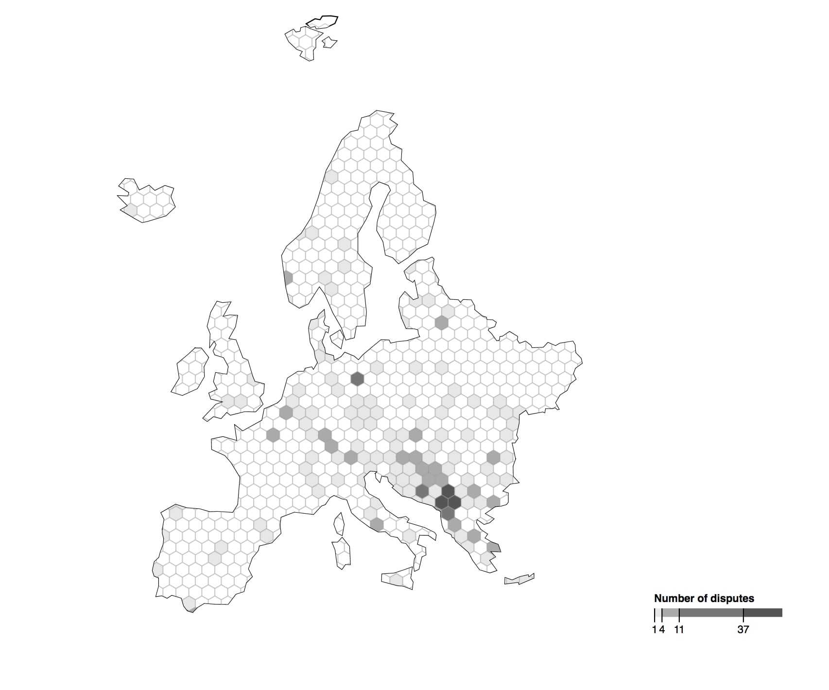
_{Data source: Midloc via data.world. Additional clip-path applied. • code}

Cities across the world

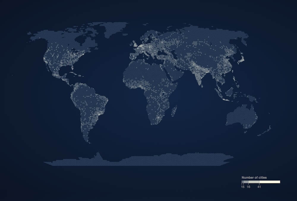
_{Data source: maxmind. Not equal area projected. • code}

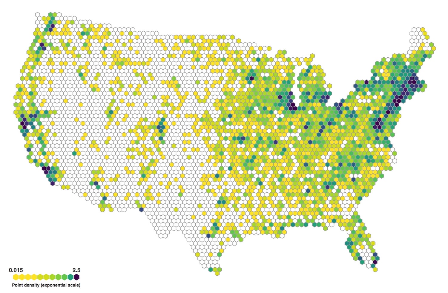
Farmers Markets in the US

_{Data source: USDA • code}

Post boxes in the UK

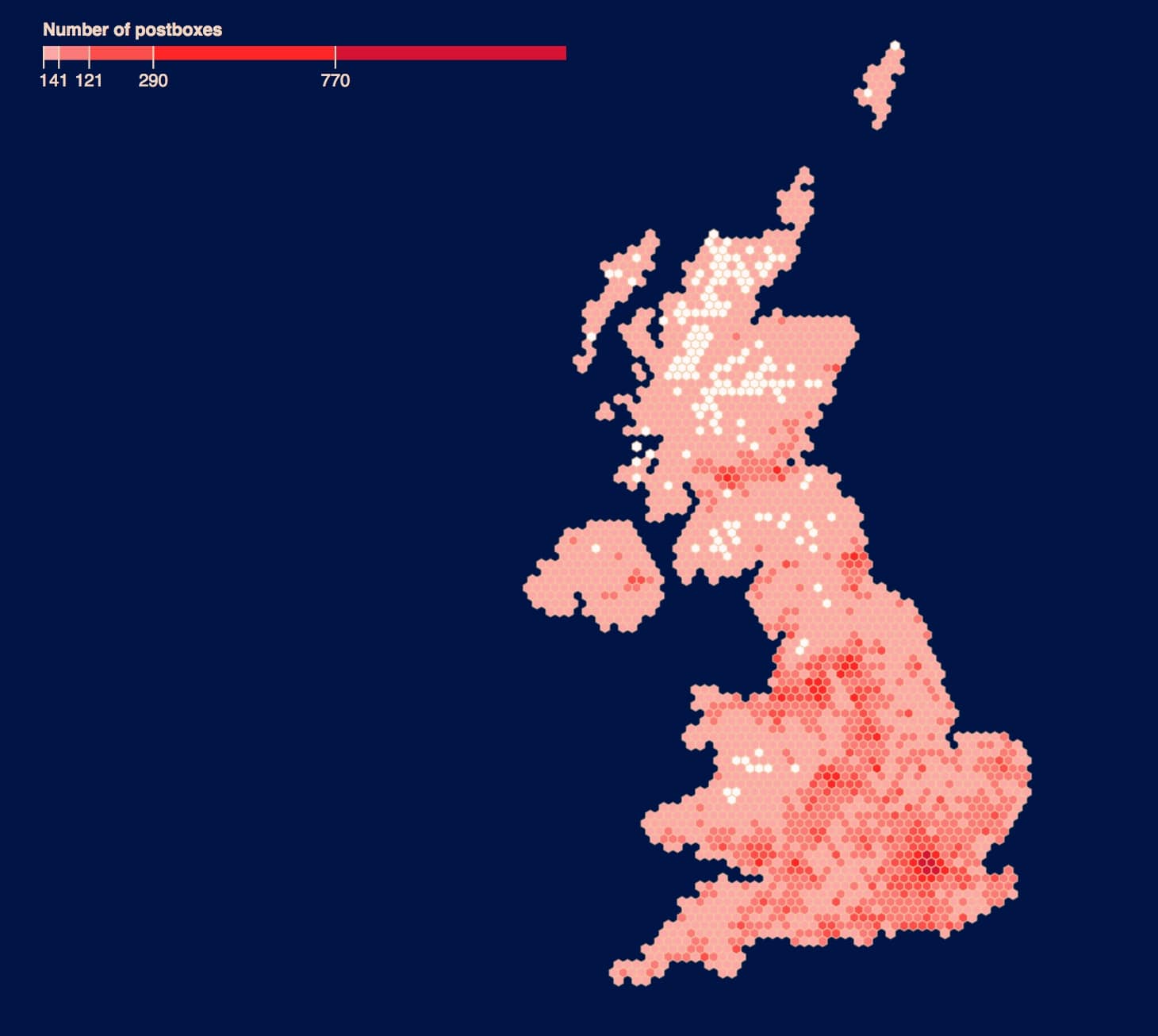
_{Data source: dracos.co.uk from here via Free GIS Data • code}

Edge Cover

The tessellation aspect might become clear in these examples. The edge cover calculation might not. In short, d3.hexgrid identifies all edge hexagons that partly lie beyond the borders of the geography, or more general: the base image presented. In a next step it calculates the edge hexagon's cover: the area the edge hexagon lies within the bounds of the base image in percent. Lastly, the point density will be calculated by:

Point density = Points in hexagon / Hexagon area in px² × Cover

A comparison:

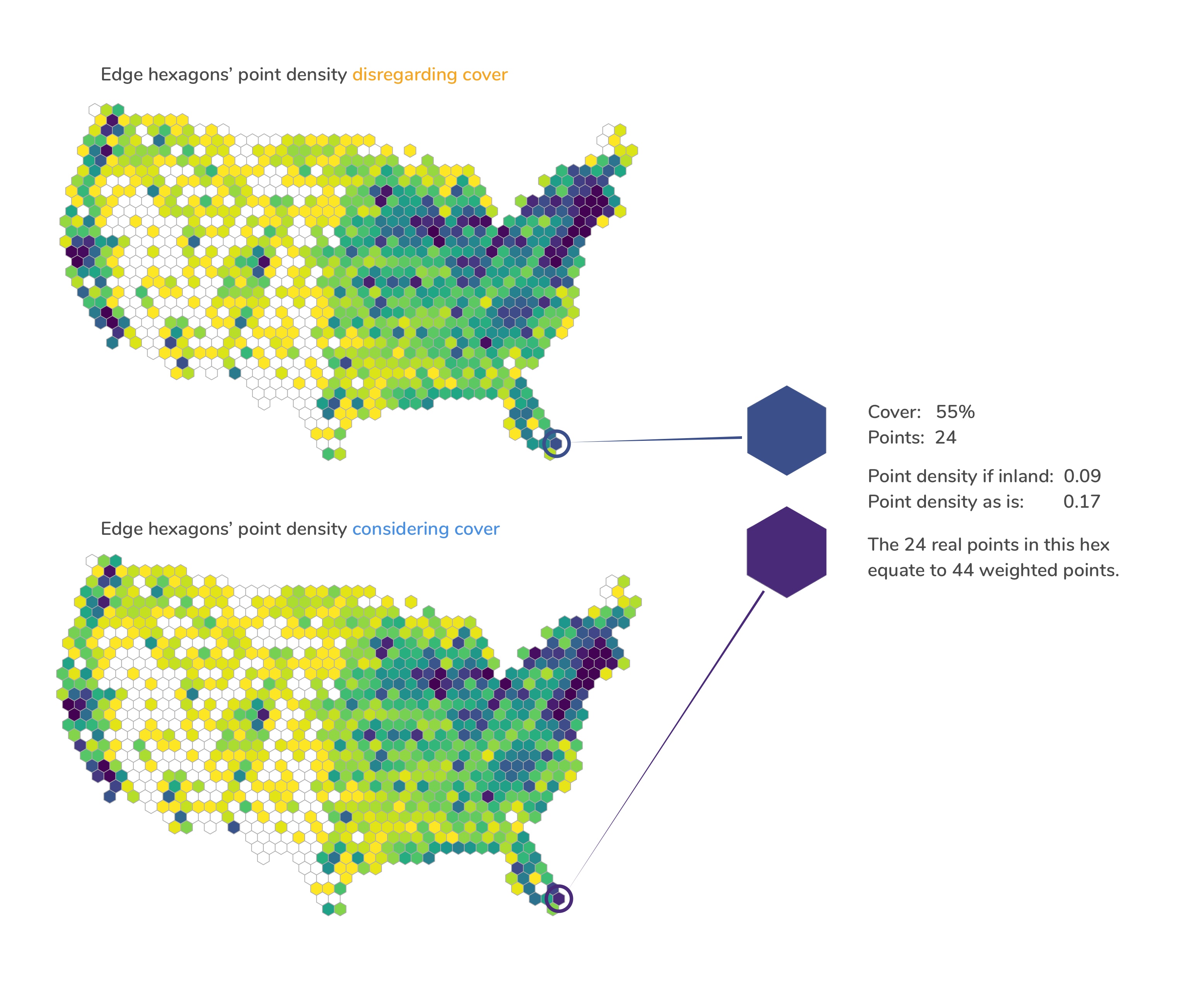
Both maps encode the number of Farmer's Markets per hexagon. Yellow represents a low, purple a high number. The edge hexagons of the upper map are not cover corrected, the edge hexagons of the lower map are.

The edge hexagon at the south-eastern tip of Florida we're comparing has a cover of 55%, meaning 55% of the hexagon's area is inland, 45% is in the Atlantic. There are a total of 22 Farmer's Markets in this hexagon. Not cover corrected, the hexagon would have a point density of 0.09 and would be filled in a dark blue with the colour scale of choice. When cover corrected, its real point density increases to 0.17 and it is coloured in a dark purple—indicating higher point density as it should.

Differences might be subtle but noticeable.

Please see the d3-hexgrid's notebook section on edge cover for a detailed description of the cover calculation.

Example usage

A lean example usage of d3-hexgrid.

// Container.
const svg = d3.select('body')
  .append('svg')
  .attr(width, 'width')
  .attr('height, 'height');

// Projection and path.
const projection = d3.geoAlbers().fitSize([width, height], geo);
const geoPath = d3.geoPath().projection(projection);

// Produce and configure the hexgrid instance.
const hexgrid = d3.hexgrid()
  .extent([width, height])
  .geography(geo)
  .projection(projection)
  .pathGenerator(geoPath);

// Get the hexbin generator and the layout.
const hex = hexgrid(myPointLocationData);

// Create a colour scale.
const colourScale = d3.scaleSequential(d3.interpolateViridis)
  .domain([...hex.grid.maxPoints].reverse());

// Draw the hexes.
svg.append('g')
  .selectAll('.hex')
  .data(hex.grid.layout)
  .enter()
  .append('path')
  .attr('class', 'hex')
  .attr('d', hex.hexagon())
  .attr('transform', d => `translate(${d.x}, ${d.y})`)
  .style('fill', d => !d.datapoints ? '#fff' : colourScale(d.datapoints));

Breaking the example down:

First, we create an SVG element. Let's assume our geography represents mainland US and comes in as a geoJSON called geo. We use an Albers projection to fit our SVG and finally get the appropriate path generator.

const svg = d3.select('body')
  .append('svg')
  .attr(width, 'width')
  .attr('height, 'height');

const projection = d3.geoAlbers().fitSize([width, height], geo);
const geoPath = d3.geoPath().projection(projection);

Next, we use d3.hexgrid() to produce a hexgrid instance we creatively call hexgrid. We immediately configure it by passing in the extent, the GeoJSON, the projection and the path-generator.

const hexgrid = d3.hexgrid()
  .extent([width, height])
  .geography(geo)
  .projection(projection)
  .pathGenerator(geoPath);

Now we can call our hexgrid instance passing in the data.

const hex = hexgrid(myPointLocationData);

This will return a hexbin generator as d3.hexbin() does, augmented with an additional object called grid, which exposes the following properties:

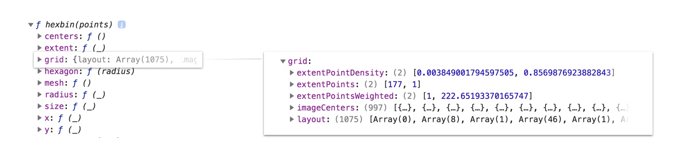
• imageCenters is an array of objects exposing at least the x, y hexagon centre coordinates of the hexgrid in screen space.

• layout is an array of arrays, each sub-array representing a hexagon in the grid. Each sub-array holds all point locations per hexagon in an object exposing at least x and y pixel coordinates as well as aggregate values. Here's an example hexagon layout sub-array with three point locations (or datapoints):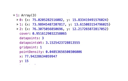

  

  The aggregate values per hexagon are:

  • cover is the percentage of this hexagon's area within the geography expressed as a number between 0 and 1.
  • datapoints is the number of points binned in the hexagon.
  • datapointsWt is the number of points weighted by the inverse cover.
  • pointDensity is the hexagon's point density.
  • gridpoint marks the hexagon as part of the initial hexgrid. This allows you to identify hexagons added by the data. Imprecise latitude and longitude data values can lead to the generation of hexagons just outside the hexgrid. d3.hexgrid will still capture and produce them. But you can spot and treat them by filtering for gridpoint === 0.
  • x and y are the hexagon centre positions in pixel coordinates.

• extentPoints is the extent of point location counts over all hexagons in the form [min number of points, max number of points].

• extentPointsWeighted is the extent of point location counts weighted by their cover over all hexagons in the form [min number of weighted points, max number of weighted points].

• extentPointDensity is the extent of cover adjusted point density over all hexagons in the form [min point density, max point density].

  These extents can be used to set a colour scale domain when encoding number of points or point density.

Working with points, for example, we might want to create the following colour scale:

const colourScale = d3.scaleSequential(d3.interpolateViridis)
  .domain([...hex.grid.maxPoints].reverse());

Here, we decide to encode the number of points per hexagon as colours along the spectrum of the Viridis colour map and create an appropriate colour scale. We reverse the extent (without modifying the original array) as we want to map the maximum value to the darkest colour, which the Viridis colour space starts with.

Finally, we build the visual:

svg.append('g')
  .selectAll('.hex')
  .data(hex.grid.layout)
  .enter()
  .append('path')
  .attr('class', 'hex')
  .attr('d', hexgrid.hexagon())
  .attr('transform', d => `translate(${d.x}, ${d.y})`)
  .style('fill', d => !d.datapoints ? '#fff' : colourScale(d.datapoints));

We use the hex.grid.layout to produce as many path's as there are hexagons—as we would with d3.hexbin()—now, however, making sure we have as many hexagons to cover our entire GeoJSON polygon. We draw each hexagon with with hexgrid.hexagon() and translate them into place. Lastly, we give our empty hexagons (!d.datapoints) a white fill and colour encode all other hexagons depending on their number of datapoints.

API Reference

# d3.hexgrid()

Constructs a hexgrid generator called hexgrid in the following. To be configured before calling it with the data you plan to visualise.

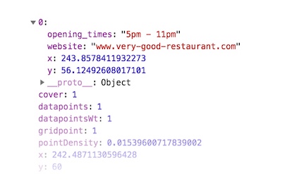
# hexgrid(data[, names])

Generates a hexbin generator augmented with a grid property, exposing the hexagon layout data as well as extents for point and point density measures. See above for the grid object's properties. Optionally names can be an array of strings, listing properties you would like to pass through from your original data to the grid layout.

Assuming you want to visualise restaurants on a map and have a restaurant dataset containing the variables website and opening_times you can say:

hexgrid(restaurantData, ['website', 'opening_times'])

As a result, objects in the hexgrid.grid.layout array will contain the two variables in addition to the default x and y coordinates:

# hexgrid.extent([extent])

Required. Sets the extent of the hexbin generator produced internally. extent can come as either a 2D array specifying top left start and bottom right end point [[x₀, y₀], [x₁, y₁]]. Alternatively extent can be specified as an array of just width and height [x₁, y₁] with the top-left corner assumed to be [0, 0]. The following two statements are equivalent:

hexgrid.extent([[0, 0], [width, height]]);
hexgrid.extent([width, height]);

# hexgrid.geography([object])

Required. object represents the base polygon for the hexgrid in GeoJSON format. If you were to project a hexgrid onto Bhutan, object would be a GeoJSON object of Bhutan.

# hexgrid.projection([projection])

Required. projection is the projection function for the previously defined geography commonly specified within the bounds of extent. See here or here for a large pond of projection functions.

# hexgrid.pathGenerator([path])

Required. path is the path generator to produce the drawing instructions of the previously defined geography based on the also previously defined projection.

# hexgrid.hexRadius([radius[, unit]])

Optional. The desired hexagon radius in pixel. Defaults to 4. unit can optionally be specified if the radius should be expressed not in pixel but in either "miles" or "kilometres". The following is valid configuration:

.hexRadius(50, 'm')   // or 'miles'
.hexRadius(50, 'km')  // or 'kilometres' or 'kilometers'

The conversion is based on a geoCircle projected in the center of the drawing area. As such the conversion can only be a proxy, however, a good one if an equal area projection is used to minimise area distortions across the geography.

# hexgrid.edgePrecision([precision])

Optional. The edge precision sets the size of the internally produced canvas to identify which area of the edge hexagon is covered by the geography. The higher the precision, the better the pixel detection at the hexagon edges. Values can be larger than 1 for small visuals. Values smaller than 0.3 will be coerced to 0.3. The default value of 1 will be fine for most purposes.

# hexgrid.gridExtend([extension])

Optional. gridExtend controls the size of the base geography. gridExtend allows you to "inflate" your hexgrid and can be used to draw more hexagons around the edges that otherwise would not be drawn.

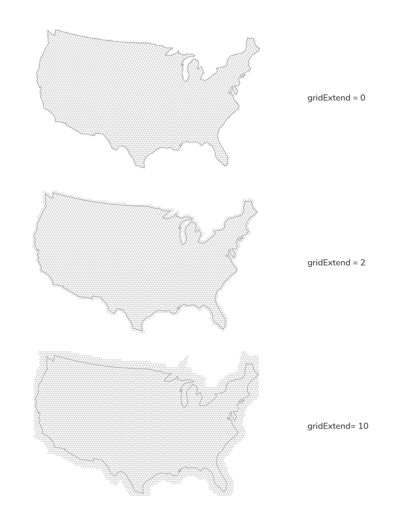
gridExtend is measured in units of hexRadius. For example, a gridExtend value of 2 would extend the grid by 2 × hexRadius pixel.

# hexgrid.geoKeys([keys])

Optional. d3.hexgrid will try to guess the key names for longitude and latitude variables in your data. The following case-insensitive key names will be sniffed out:

• longitude, long, lon, lng, lambda as well as
• latitude, lat and phi.

If you choose other names like for example upDown and leftRight, you have to specify them as hexgrid.geokeys(['upDown', 'leftRight']) with the first element representing longitude and the second latitude.

Don't call your geo keys x or y or otherwise include x and/or y keys in your passed in user variables as they are reserved keys for the pixel coordinates of the layout.

Helper functions

The following functions can be helpful to filter out point location data that lie beyond the base geography.

# d3.geoPolygon([geo, projection])

Transforms a GeoJSON geography into a Polygon or MultiPolygon. geo is a GeoJSON of the base geography. projection is the applied projection function.

# d3.polygonPoints([data, polygon])

data is an array of point location objects with x and y properties in screen space. polygon is a Polygon or MultiPolygon as produced by d3.geoPolygon(). Returns a new array of point location objects exclusively within the bounds of the specified polygon.

If you had a point location dataset of all post boxes in the world, but you only want to visualise UK post boxes you can use these helper functions to produce a dataset with only UK post boxes like so:

const polygonUk   = d3.geoPolygon(ukGeo, projectionUk);
const postboxesUk = d3.polygonPoints(postboxesWorld, polygonUk);

If you plan to use the d3-hexgrid produced extents in a color scale, it is suggested to focus your dataset on your base geography. If produced with data beyond your base geography, the extents might not be meaningful.

General notes on hexagonal binning

Hexagons are often ideal for binning point location data as they are the shape closest to circles that can be regularly tessellated. As a result, point distributions binned by a hexagon are relatively spike-less and neighbouring hexagons are equidistant.

While being the right choice in many cases, two notes should be considered when using hexagonal binning—or any point location binning for that matter:

Use equal area projections for the base geography.

The world is something like a sphere and there are numerous ways to project a sphere onto a 2D plane. The projection used has an important effect on the analysis. Any tessellation normalises space to equally sized units—hexagons in this case—which invites the reader to assume that each unit covers the same area. However, some projections, like the ubiquitous Mercator projection, will distort area increasingly towards the poles:

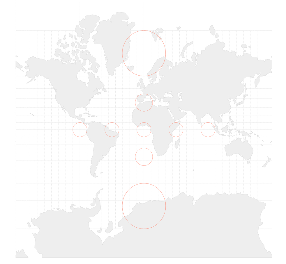
_{Source: D3 in depth by Peter Cook}

All red circles on above map are of the same area. As a result, tessellating a Mercator world map with hexagons will produce many more hexagons per square mile in Norway compared to Brazil, for example.

Equal area projections will help to avoid this problem to a large extent.

Consciously choose the hexagon radius size.

Location binning is susceptible to the Modifiable Areal Unit Problem. The MAUP—or more specifically the zonal MAUP—states that a change in size of the analysis units can lead to different results. In other words, changing the hexagons’ size can produce significantly different patterns—although the views across different sizes share the same data. Awareness is the only corrective to the MAUP. As such, it is recommended to test a few unit sizes before consciously settling for one, stating the reasons why and/or allowing the readers to see or chose different hexagon sizes.

Thanks!

A big thanks to Philippe Rivière for bringing the grid layout algorithm on track and sparking the idea for the edge cover calculation. This plug-in would look different and be significantly less performant without his elegant ideas.

For a deeper dive read Amit Patel's (aka reblobgames) seminal hexagon tutorial. The best to find out there. Also see the great things Uber's been doing with H3, which in many ways goes far beyond this plugin.