![]()


Bertin.js is a JavaScript library for visualizing geospatial data and make thematic maps for the web.
The project is under active development. Some of features and options are subject to change. We welcome contributions of all kinds: bug reports, code contributions and documentation. A todo list of the next improvements is available here.

- Introduction
- Who is Bertin?
- Installation
- Usage
- Drawing a map
- Map types
- Map components
- Custom Layer
- Geojson properties selections
- Other functions
- Update function
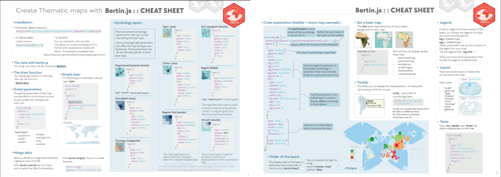
- Bonus: a cheat sheet
bertin is an easy to use JavaScript library mainly based on D3.js makes creating thematic maps simple. The principle is to work with layers stacked on top of one other. Much like in Geographic Information Software (GIS) software, Bertin.js displays layers with a specific hierarchy. The layer at bottom are rendered and then followed by the layer right above it. Some of the layers are used to display various components of a map, some of common layers are: header, footer, graticule, outline, choro, typo, prop, shadow, scalebar, text etc.
- The
draw()function is the most important function of the library. It allows you to draw all types of maps. - The
update()function allows you to modify specific elements of the map without the need to redraw everything. Only the parameters underlined in the documentation can be modified through this function.
Cheat Sheet
Who is Bertin? {#who-is-bertin}
Jacques Bertin (1918-2010) was a French cartographer, whose major contribution was a theoretical and practical reflection on all graphic representations (diagrams, maps and graphs), forming the subject of a fundamental treatise, Graphic Semiology, originally published in 1967. Bertin's influence remains strong not only in academics, teaching of cartography today, but also among statisticians and data visualization specialists.
Installation {#installation}
In browser
Latest version
<script
  src="https://cdn.jsdelivr.net/npm/bertin"
  charset="utf-8"
></script>
Pinned version
<script src="https://cdn.jsdelivr.net/npm/bertin@1.7" charset="utf-8"></script>In Observable
Latest version
bertin = require("bertin");Pinned version
bertin = require("bertin@1.7");In Quarto
In Quarto, you can use bertin with ojs cells. This allows to combine analyses in R or Python with visualizations made with bertin. An example is available here
Usage {#usage}
In browser
<script src="https://cdn.jsdelivr.net/npm/d3@7"></script>
<script src="https://cdn.jsdelivr.net/npm/bertin"></script>

<script>
  let geojson =
    "https://raw.githubusercontent.com/neocarto/bertin/main/data/world.geojson";

  d3.json(geojson).then((r) =>
    document.body.appendChild(
      bertin.draw({
        params: {
          projection: "VanDerGrinten4",
          clip: true,
        },
        layers: [
          { geojson: r, tooltip: ["$ISO3", "$NAMEen"] },
          { type: "outline" },
          { type: "graticule" },
        ],
      })
    )
  );
</script>
See examples: Example 1, Example 2 and Example 3.
In Observable Notebook
The bertin.js library is really easy to use within an Observable notebook. You'll find many examples in this notebook collection. Feel free to fork, copy, modify with your own data.
Drawing a map {#drawing-a-map}
draw() is the main function of the library. It allows you to make various thematic maps. It allows to display and overlay different types of layers listed below. The layers written on top are displayed first. Source Example
Global parameters
In the section params, we define the global parameters of the map: its size, projection, background color, etc. To have access to a large number of projections, you will need to load the d3-geo-projection@4 library. This section is optional.
Code
bertin.draw({
  params: {
    projection: d3.geoBertin1953(),
    width: 750,
  },
  layers: [...]
})
A globe view is available for some types of layers: simple (with symbol_shift == 0), spikes, bubble (with dorling == true), geolines, graticule, inner, missing, shadow, tissot, dotdensity and label.
To use it, you juste have to use "globe" as projection. You can also define the center og the map by using "globe(x,y,rotate)"
Parameters
- projection: a d3 function or string defining the map projection. Refer d3-geo-projection and spatialreference.org for more detailed explanation. (default: d3.geoEquirectangular() except if you use tiles. in this case, the projection is automatically set to d3.geoMercator()). Moreover, if you define projection as "user", you can display a basemap already projected. Example. Note alsa that custom projections are available. Try "Polar", "Spilhaus" or "HoaXiaoguang".
- width: width of the map (default:1000);
-
extent: a feature or a bbox array defining the extent e.g. a country or
[[112, -43],[153, -9]](default: null) - margin: margin around features to be displayed. You can specify a single value or an array [top, right, bottom, left]. (default: 1)
- background: color of the background (default: "none")
- clip: a boolean to avoid artifacts of discontinuous projection (default: "false")
- reverse: a boolean. By default, the layer placed on the top of the code is display on the top of the map. With reverse = true, your can reverse this order (default: false).
Map types {#map-types}
Simple layer
The layer type allows to display a simple geojson layer (points, lines or polygons). Source. Example 1 and Example 2.

Code
bertin.draw({
  layers: [
    {
      type: "layer",
      geojson: *a geojson here*,
      fill: "#e6acdf",
    }
  ]
})
Parameters
-
geojson: a geojson (compulsory)
-
rewind: a boolean. If true, the geojson is rewinded for a proper display (default: false)
-
fill
: fill color (default: a random color)
-
stroke
: stroke color (default: "white")
-
strokeWidth
stroke width (default:0.5)
-
strokeLinecap
: stroke-linecap (default:"round")
-
strokeLinejoin
: stroke-linejoin (default:"round")
-
strokeDasharray
: stroke-dasharray (default:"none")
-
fillOpacity
: fill opacity (default:1)
-
strokeOpacity
: stroke opacity (default:1)
-
symbol
: if it is a dot layer, the type of symbol. "circle", "cross", "diamond", "square", "star", "triangle", "wye" (default: "circle")
-
symbol_size
: if it is a dot layer, a number indicating the size of the symbol (default: 5)
-
symbol_shift: if it is a dot layer, use a value > 0 to switch symbols and avoid overlay (default: 0)
-
symbol_iteration: Number of iteration to shift symbols (default: 200)
-
viewof: Boolean to use this layer as an Observable view. See explanations (default: false)
Parameters of the legend
- leg_x: position in x (if this value is not filled, the legend is not displayed)
- leg_y: position in y (if this value is not filled, the legend is not displayed)
- leg_w: width of the box (default: 30)
- leg_h: height of the box (default: 20)
- leg_title: title of the legend (default: null)
- leg_text: text of the box (default: "leg_text")
- leg_fontSize: title legend font size (default: 14)
- leg_fontSize2: values font size (default: 10)
- leg_fill: color of the box (same as the layer displayed)
- leg_stroke: stroke of the box (default: "black")
- leg_strokeWidth: stroke-width (default: 0.5)
- leg_fillOpacity: stroke opacity (same as the layer displayed)
- leg_txtcol: color of the text (default: "#363636")
Choropleth
The choro type aims to draw Choropleth maps. This kind of representation is especially suitable for relative quantitative data (rates, indices, densities). The choro type can be applied to the fill or stroke property of a simple layer. Example.

Code
bertin.draw({
  layers: [
    {
      type: "layer",
      geojson: data,
      fill: {
        type: "choro",
        values: "gdppc",
        nbreaks: 5,
        method: "quantile",
        colors: "RdYlGn",
        leg_round: -1,
        leg_title: `GDP per inh (in $)`,
        leg_x: 100,
        leg_y: 200
      }
  ]
})
Parameters
-
values
: a string corresponding to the targeted variable in the properties (compulsory)
-
nbreaks
: Number of classes (default:5)
-
breaks
: Class breaks (default:null)
-
colors
: An array of colors or a palette of colors (Blues", "Greens", "Greys", "Oranges", "Purples", "Reds", "BrBG", "PRGn", "PiYG", "PuOr", "RdBu", "RdYlBu", "RdYlGn", "Spectral","Turbo","Viridis","Inferno", "Magma", "Plasma", "Cividis", "Warm", "Cool", "CubehelixDefault", "BuGn", "BuPu", "GnBu", "OrRd", "PuBuGn", "PuBu", "PuRd", "RdPu", "YlGnBu", "YlGn", "YlOrBr", "YlOrRd", "Rainbow", "Sinebow". default: Blues) See
-
method
: A method of classification. "quantile", "q6", "equal", "msd" (mean standard deviation), "jenks", "geometric", "headtail" or "pretty" (default: "quantile"). See statsbreaks example for method implementation in action.
-
middle
: for msd method only. middle class or not (default:false);
-
k
: for msd method only. number of sd. (default:1);
-
col_missing
: Color for missing values (default "#f5f5f5")
-
txt_missing
: Text for missing values (default "No data")
-
stroke
: stroke color (default: "white")
-
strokeWidth
: Stroke width (default: 0.5)
-
fillOpacity
: Fill opacity (default: 1)
Parameters of the legend
-
leg_x
: position in x (if this value is not filled, the legend is not displayed)
-
leg_y
: position in y (if this value is not filled, the legend is not displayed)
-
leg_w
: width of the box (default: 30)
-
leg_h
: height of the box (default:20)
-
leg_text
: text of the box (default: "leg_text")
-
leg_fontSize
: text font size (default: 10)
-
leg_fill
: color of the box (same as the layer displayed)
-
leg_stroke
: stroke of the box (default: "black")
-
leg_strokeWidth
: stroke-width (default: 0.5)
-
leg_fillOpacity
: stroke opacity (same as the layer displayed)
-
leg_txtcol
: color of the text (default: "#363636")
-
leg_round
: Number of digits (default: undefined)
Typology
The typo type allows to realize a qualitative map. The choro type can be applied to the fill or stroke property of a simple layer. Example.

Code
bertin.draw({
  layers: [
    {
      type: "layer",
      geojson: data,
      fill: {
        type: "typo",
        values: "region",
        pal: "Tableau10",
        tooltip: ["$region", "$name"],
        leg_title: `The Continents`,
        leg_x: 55,
        leg_y: 180
      }
    }
  ]
})
Parameters
-
values
: a string corresponding to the targeted variable in the properties (compulsory)
-
colors
: An array containing n colors for n types, or a a palette of categorical colors (default: "Tableau10"). See the handy color scheme reference for full list of palettes.
-
order
: an array of values to set the order of the colors
-
col_missing
: Color for missing values (default "#f5f5f5")
-
txt_missing
: Text for missing values (default "No data")
-
stroke
: stroke color (default: "white")
-
strokeWidth
: Stroke width (default: 0.5)
-
fillOpacity
: Fill opacity (default: 1)
Parameters of the legend
-
leg_x
: position in x (if this value is not filled, the legend is not displayed)
-
leg_y
: position in y (if this value is not filled, the legend is not displayed)
-
leg_w
: width of the box (default: 30)
-
leg_h
: height of the box (default:20)
-
leg_title
: title of the legend (default; null)
-
leg_fontSize
: title legend font size (default: 14)
-
leg_fontSize2
: values font size (default: 10)
-
leg_stroke
: stroke of the box (default: "black")
-
leg_strokeWidth
: stroke-width (default: 0.5)
-
leg_fillOpacity
: stroke opacity (same as the layer displayed)
-
leg_txtcol
: color of the text (default: "#363636")
Bubble
The bubble type is used to draw a map by proportional circles. Source, Example.

Code
bertin.draw({
  layers: [
    {
      type: "bubble",
      geojson: countries,
      values: "pop",
      k: 60,
      tooltip: ["$country", "$pop", "(inh.)"],
    },
  ],
});
Parameters
-
geojson: a geojson (compulsory)
-
rewind: a boolean. If true, the geojson is rewinded for a proper display (default: false)
-
values
: a string corresponding to the targeted variable in the properties(compulsory)
-
k
: size of the largest circle (default:50)
-
fixmax: Max value to fix the size of the biggest circle, in order to make maps comparable (default:undefined)
-
fill
: fill color (default: random color)
-
stroke
: stroke color (default: "white")
-
strokeWidth
: stroke width (default: 0.5)
-
fillOpacity
: fill opacity (default: 1)
-
dorling
: a boolean (default:false)
-
iteration: an integer to define the number of iteration for the Dorling method (default: 200)
-
tooltip: an array of values defining what to display within the tooltip. If you use a $, the value within the geojson is displayed. Example.
-
viewof: Boolean to use this layer as an Observable view. See explanations (default: false)
Parameters of the legend
- leg_x: position in x (if this value is not filled, the legend is not displayed)
- leg_y: position in y (if this value is not filled, the legend is not displayed)
- leg_fill: color of the circles (default: "none")
- leg_stroke: stroke of the circles (default: "black")
- leg_strokeWidth: stoke-width (default: 0.8)
- leg_txtcol: color of the text (default: "#363636")
- leg_title: title of the legend (default var_data)
- leg_round: number of digits after the decimal point (default: undefined)
- leg_divisor: A number to divide to the values in the legend. For example, 1000 is used to convert units to thousands. 1000000 allows to convert units into millions (default: 1).
- leg_fontSize: title legend font size (default: 14)
- leg_fontSize2: values font size (default: 10)
Square
The square type is used to draw a map by proportional squares. Source, Example.

Code
bertin.draw({
  layers: [
    {
      type: "square",
      geojson: countries,
      values: "pop",
      k: 60,
      tooltip: ["$country", "$pop", "(inh.)"],
    },
  ],
});
Parameters
-
geojson: a geojson (compulsory)
-
rewind: a boolean. If true, the geojson is rewinded for a proper display (default: false)
-
values
: a string corresponding to the targeted variable in the properties(compulsory)
-
k
: size of the largest circle (default:50)
-
fixmax: Max value to fix the size of the biggest circle, in order to make maps comparable (default:undefined)
-
fill
: fill color (default: random color)
-
stroke
: stroke color (default: "white")
-
strokeWidth
: stroke width (default: 0.5)
-
fillOpacity
: fill opacity (default: 1)
-
demers
: a boolean to avoid overlay. Dorling parameter works also (default:false) - EXPERIMENTAL
-
iteration: an integer to define the number of iteration for the Dorling method (default: 200)
-
tooltip: an array of values defining what to display within the tooltip. If you use a $, the value within the geojson is displayed. Example.
-
viewof: Boolean to use this layer as an Observable view. See explanations (default: false)
Parameters of the legend
- leg_x: position in x (if this value is not filled, the legend is not displayed)
- leg_y: position in y (if this value is not filled, the legend is not displayed)
- leg_fill: color of the circles (default: "none")
- leg_stroke: stroke of the circles (default: "black")
- leg_strokeWidth: stoke-width (default: 0.8)
- leg_txtcol: color of the text (default: "#363636")
- leg_title: title of the legend (default var_data)
- leg_round: number of digits after the decimal point (default: undefined)
- leg_divisor: A number to divide to the values in the legend. For example, 1000 is used to convert units to thousands. 1000000 allows to convert units into millions (default: 1).
- leg_fontSize: title legend font size (default: 14)
- leg_fontSize2: values font size (default: 10)
Regular Bubble
The regularbubble type is used to draw a map by proportional circles in a regular grid, from absolute quantitative data. Source, Example and methodology.

Code
bertin.draw({
  layers: [
    {
      type: "regularbubble",
      geojson: countries,
      step:20,
      values: "pop",
      k: 60,
      tooltip: "$value",
    },
  ],
});
Parameters
- step: Gap between the points (default:20)
- operator: "sum" for absolute quantitative data or "mean" for relative data (default: "sum". highly recommended)
- geoprocessing: "intersection" (intersection between polygons and grid squares. Assignment of values in proportion to the intersected area) or "dotinpoly" (considers each grid square and assigns the value of the underlying polygon or the weighted average of intersecting polygons. ). (Default: "intersection")
- blur: radius of the kernel defined in d3.blur2 (default: 0)
All other parameters are the same as for the bubble layer
Regular Square
The regularsquare type is used to draw a map by proportional squares in a regular grid, from absolute quantitative data. Source, Example and methodology.

Code
bertin.draw({
  layers: [
    {
      type: "regularsquare",
      geojson: countries,
      step:20,
      values: "pop",
      k: 60,
      tooltip: "$value",
    },
  ],
});
Parameters
- step: Gap between the points (default:20)
- operator: "sum" for absolute quantitative data or "mean" for relative data (default: "sum". highly recommended)
- geoprocessing: "intersection" (intersection between polygons and grid squares. Assignment of values in proportion to the intersected area) or "dotinpoly" (considers each grid square and assigns the value of the underlying polygon or the weighted average of intersecting polygons. ). (Default: "intersection")
- blur: radius of the kernel defined in d3.blur2 (default: 0)
All other parameters are the same as for the square layer
Regular grid
The regulargrid type is a way to transform an irregular geographic mesh into a regular mesh. The values of the grid cells are obtained in proportion to the intersected surface. This representation mode is only suitable for absolute quantitative data. But you can use 2 quantitative data to compute a ratio Source, Example and methodology.

Code
bertin.draw({
  layers: [
    {
      type: "regulargrid",
      geojson: countries,
      step:20,
      values: "pop",
      fill:{
        nbreaks: 6,
        method: "quantile",
        colors: "Blues"
      }
      tooltip: "$value",
    },
  ],
});
Parameters
- step: Gap between the points (default:20)
- operator: "sum" for absolute quantitative data or "mean" for relative data (default: "sum")
- geoprocessing: "intersection" (intersection between polygons and grid squares. Assignment of values in proportion to the intersected area) or "dotinpoly" (considers each grid square and assigns the value of the underlying polygon or the weighted average of intersecting polygons. ). (Default: "intersection")
- blur: radius of the kernel defined in d3.blur2 (default: 0)
All other parameters are the same as for choropleth maps
Stock and ratio
In thematic mapping, we often have to represent an absolute quantitative data with a size variation and relative quantitative data with color variations. For this we can use the bubble type and the choro type together. Example.

Code
bertin.draw({
  params: { projection: d3.geoPolyhedralWaterman() },
  layers: [
    {
      type: "bubble",
      geojson: data,
      leg_round: -2,
      values: "pop",
      fill: {
        type: "choro",
        method: "quantile",
        nbreaks: 5,
        values: "gdppc",
        pal: "RdYlGn",
      },
    },
  ],
});
Stock and typo
In thematic mapping, we often have to represent an absolute quantitative data with a size variation and relative quantitative data with color variations. For this we can use the bubble type and the typo type together. Example.

Code
bertin.draw({
  layers: [
    {
      type: "bubble",
      geojson: data,
      values: "pop",
      fill: {
        type: "typo",
        values: "region",
      },
    },
  ],
});
Dorling cartogram
The dorling parameter can be used with the bubble type to design a Dorling cartogram. Example.

Code
bertin.draw({
  layers: [
    {
      type: "bubble",
      geojson: data,
      values: "pop",
      k: k,
      dorling: true,
      iteration: 100,
      fill: "#E95B40",
    },
  ],
});
Dot cartogram
The dotcartogram type is a method of map representation that follows Dorling's cartograms and dot density maps. The data from each territorial unit are dissolved in such a way that a dot represents a constant quantity, the same on the whole map. Source Example.

Code
bertin.draw({
  params: { projection: d3.geoBertin1953() },
  layers: [
    {
      type: "dotcartogram",
      geojson: data,
      onedot: 200000000000,
      iteration: 200,
      values: "gdp",
      radius: radius,
      span: span,
      leg_fill: "none",
      leg_stroke: "black",
      leg_strokeWidth: 1.5,
      leg_x: 800,
      leg_y: 450,
      leg_title: `GDP by world region`,
      leg_txt: "200 billion $",
      fill: "red",
      tooltip: ["$name", "$region"],
    },
  ],
});
Parameters
- geojson: a geojson (compulsory)
- rewind: a boolean. If true, the geojson is rewinded for a proper display (default: false)
- values: a string corresponding to the targeted variable in the properties(compulsory)
- radius: radius of dots (default:4)
- nbmax: number max of circles on the map (default:200)
- onedot: dot value (if onedot is filled, nbmax is useless)
- span: spacing between dots (default 0.5)
- fill: fill color (default: random color)
- stroke: stroke color (default: "white")
- strokeWidth: stroke width (default: 0.5)
- fillOpacity: fill opacity (default: 1)
- tooltip an array of values defining what to display within the tooltip. If you use a $, the value within the geojson is displayed.
- iteration an integer to define the number of iteration for the Dorling method (default 200)
- viewof: Boolean to use this layer as an Observable view. See explanations (default: false)
Parameters of the legend
- leg_x: position in x (if this value is not filled, the legend is not displayed)
- leg_y: position in y (if this value is not filled, the legend is not displayed)
- leg_fill: color of the circles (default: "none")
- leg_stroke: stroke of the circles (default: "black")
- leg_strokeWidth: stoke-width (default: 0.8)
- leg_txtcol: color of the text (default: "#363636")
- leg_title: title of the legend (default var_data)
- leg_txt: text in the legend (default onedot value)
- leg_fontSize: title legend font size (default: 14)
- leg_fontSize2: text font size (default: 10)
Mushroom
The mushroom type is used to draw a map with 2 superposed proportional semi-circles. This type of representation can be used when two data with the same order of magnitude need to be compressed. Source, Example.

Code
bertin.draw({
  layers: [
    {
      type: "mushroom",
      geojson: mygeojson,
      top_values: "gdp_pct",
      bottom_values: "pop_pct",
      bottom_tooltip: ["name", "pop", "(thousands inh.)"],
      top_tooltip: ["name", "gdp", "(million $)"],
    },
  ],
});
Parameters
- geojson: a geojson (compulsory)
- rewind: a boolean. If true, the geojson is rewinded for a proper display (default: false)
- top_values: a string corresponding to the targeted top variable in the properties (compulsory)
- bottom_values: a string corresponding to the targeted bottom variable in the properties(compulsory)
- top_fill: top fill color (default: "#d64f4f")
- bottom_fill: bottom fill color (default: "#4fabd6")
- k: size of the largest semi circle (default:50)
- stroke: stroke color (default: "white")
- strokeWidth: stroke width (default: 0.5)
- fillOpacity: fill opacity (default: 1)
- strokeOpacity: stroke opacity (default: 1)
- top_tooltip: an array of values defining what to display within the tooltip. If you use a $, the value within the geojson is displayed.
- bottom_tooltip: an array of values defining what to display within the tooltip. If you use a $, the value within the geojson is displayed.
- viewof: Boolean to use this layer as an Observable view. See explanations (default: false)
Parameters of the legend
- leg_x: position in x (if this value is not filled, the legend is not displayed)
- leg_y: position in y (if this value is not filled, the legend is not displayed)
- leg_fontSize: title legend font size (default: 14)
- leg_fontSize2: values font size (default: 10)
- leg_round: number of digits after the decimal point (default: undefined)
- leg_txtcol: color of the text (default: "#363636")
- leg_title: title of the legend (default "Title, year")
- leg_stroke: stroke of the circles (default: "black")
- leg_top_txt title for the top variable (default top_var)
- leg_bottom_txt title for the bottom variable (default bottom_var)
- leg_top_fill color of top semi circles (default same as top_fill)
- leg_bottom_fill color of bottom semi circles (default same as bottom_fill)
- leg_strokeWidth stroke width of elements in the legend (default 0.8)
Dot Density
The dotdensity type allows to display a doty density layer geojson layer from polygons and attribute data. Source. Example

Code
bertin.draw({
  layers: [
    {
      type: "dotdensity",
      geojson: *a geojson here (polygon)*,
      values: *a fiel here*
      dotvalue: *a number*,
    }
  ]
})
Parameters
- geojson: a geojson polygons or Multipolygons (compulsory)
- rewind: a boolean. If true, the geojson is rewinded for a proper display (default: false)
- values: a string corresponding to the targeted variable in the properties(compulsory)
- dotvalue: a number representing the value of each point (default: a computed number so that there are no more than 1000 dots on the map.)
- fill: fill color (default: a random color)
- stroke: stroke color (default: "white")
- strokeWidth stroke width (default:0.5)
- fillOpacity: fill opacity (default:1)
- strokeOpacity: stroke opacity (default:1)
- symbol: if it is a dot layer, the type of symbol. "circle", "cross", "diamond", "square", "star", "triangle", "wye" (default: "circle")
- symbol_size: if it is a dot layer, a number indicating the size of the symbol (default: 5)
- symbol_shift: if it is a dot layer, use a value > 0 to switch symbols and avoid overlay (default: 0)
- symbol_iteration: Number of iteration to shift symbols (default: 200)
Parameters of the legend
- leg_x: position in x (if this value is not filled, the legend is not displayed)
- leg_y: position in y (if this value is not filled, the legend is not displayed)
- leg_w: width of the box (default: 30)
- leg_h: height of the box (default:20)
- leg_title: title of the legend (default: null)
- leg_text: text in the legend (default: dot value)
- leg_fontSize: title legend font size (default: 14)
- leg_fontSize2: values font size (default: 10)
- leg_fill: color of the box (same as the layer displayed)
- leg_stroke: stroke of the box (default: "black")
- leg_strokeWidth: stroke-width (default: 0.5)
- leg_fillOpacity: stroke opacity (same as the layer displayed)
- leg_txtcol: color of the text (default: "#363636")
Spikes
The spikes type is used to draw a map with spikes. Source, Example.

Code
bertin.draw({
  layers: [
    {
      type: "spikes",
      geojson: countries,
      values: "pop",
      k: 60,
      w: 8,
      tooltip: ["$country", "$pop", "(inh.)"],
    },
  ],
});
Parameters
-
geojson: a geojson (compulsory)
-
rewind: a boolean. If true, the geojson is rewinded for a proper display (default: false)
-
values
: a string corresponding to the targeted variable in the properties(compulsory)
-
k
: height of the highest peak (default:50)
-
w: width of the spikes (default:10)
-
fill
: fill color (default: #a31d88)
-
stroke
: stroke color (default: #a31d88)
-
strokeWidth
: stroke width (default: 0.7)
-
fillOpacity
: fill opacity (default: 0.3)
-
tooltip an array of values defining what to display within the tooltip. If you use a $, the value within the geojson is displayed.
-
viewof: Boolean to use this layer as an Observable view. See explanations (default: false)
Parameters of the legend
- leg_x: position in x (if this value is not filled, the legend is not displayed)
- leg_y: position in y (if this value is not filled, the legend is not displayed)
- leg_fill: color of the circles (default: "none")
- leg_stroke: stroke of the circles (default: "black")
- leg_strokeWidth: stoke-width (default: 0.8)
- leg_txtcol: color of the text (default: "#363636")
- leg_title: title of the legend (default var_data)
- leg_round: rounding (default: undefined)
- leg_fontSize: title legend font size (default: 14)
- leg_fontSize2: values font size (default: 10)
Ridge
The ridge type allows to produce 2.5D maps by varying the height of lines. The method takes as input polygons or multi polygons. Source Example.

Code
bertin.draw({
  layers: [
 {
      type: "ridge",
      geojson: data,
      values: "pop",
      step: 30,
      blur: 0.4,
      k: 50
    },
  ],
});
Parameters
-
geojson: a geojson (compulsory)
-
rewind: a boolean. If true, the geojson is rewinded for a proper display (default: false)
-
values: a string corresponding to the targeted variable in the properties
-
stroke
: stroke color (default: "white")
-
strokeWidth stroke width (default: 0.5)
-
fillOpacity
: fill opacity (default: 1)
-
strokeOpacity
: stroke opacity (default: 1)
-
strokeDasharray
: stroke-dasharray (default: "none")
-
step: Gap between the points (default: 20)
-
k: Height of lines (default: 100)
-
operator: "sum" for absolute quantitative data or "mean" for relative data (default: "mean")
-
geoprocessing: "intersection" (intersection between polygons and grid squares. Assignment of values in proportion to the intersected area) or "dotinpoly" (considers each grid square and assigns the value of the underlying polygon or the weighted average of intersecting polygons. ). (Default: "dotinpoly")
-
blur: radius of the kernel defined in d3.blur2 (default: 0.4)
Smooth
The smooth type (or heatmap or contour) is a way to produce a continuous représentations from quantitative data. The algorithm is complex. The values produced do not really make sense. Explanations with the parameters. Source, Example and methodology.

Code
bertin.draw({
  layers: [
 {
      type: "smooth",
      geojson: data,
      values: "pop",
      thresholds: 50,
      bandwidth: 25,
      colorcurve: 1,
    },
  ],
});
Parameters
- geojson: a geojson (compulsory)
- rewind: a boolean. If true, the geojson is rewinded for a proper display (default: false)
- values: a string corresponding to the targeted variable in the properties
- stroke: stroke color (default: "white")
- strokeWidth stroke width (default:0.5)
- strokeLinecap: stroke-linecap (default:"round")
- strokeLinejoin: stroke-linejoin (default:"round")
- strokeDasharray: stroke-dasharray (default:"none")
- fillOpacity: fill opacity (default:1)
- strokeOpacity: stroke opacity (default:1)
Contour parameters
- fill: color palette. "Blues", "Greens", "Greys", "Oranges", "Purples", "Reds", "BrBG", "PRGn", "PiYG", "PuOr", "RdBu", "RdYlBu", "RdYlGn", "Spectral","Turbo","Viridis","Inferno", "Magma", "Plasma", "Cividis", "Warm", "Cool", "CubehelixDefault", "BuGn", "BuPu", "GnBu", "OrRd", "PuBuGn", "PuBu", "PuRd", "RdPu", "YlGnBu", "YlGn", "YlOrBr", "YlOrRd", "Rainbow", "Sinebow". (default: RdYlGn)
- thresholds: number of classes (default: 100)
- bandwidth: bandwidth (the standard deviation) of the Gaussian kernel and returns the estimate. (default: 5)
- colorcurve: a value to curve the color interpolation (default: 2)
- reverse: a boolean reverse the colors (default: false)
- remove: number of polygons to remove (default: 0)
- clip: a boolean to clip the contours with the input geojson (default: false)
By default, the smooth layer is calculated from dots or centroids. But it is possible to go through a regular grid by using theses parameters.
- grid_step: Gap between the points (default:20)
- grid_blur: radius of the kernel defined in d3.blur2 (default: 0)
- grid_operator: "sum" for absolute quantitative data or "mean" for relative data (default: "sum". highly recommended)
- grid_geoprocessing: "intersection" (intersection between polygons and grid squares. Assignment of values in proportion to the intersected area) or "dotinpoly" (considers each grid square and assigns the value of the underlying polygon or the weighted average of intersecting polygons. ). (Default: "intersection")
Thickness
On each layer, you can dynamically vary the thickness of the paths. This can be useful to make for example flow maps or discontinuity maps. Source
Code - Constant Thickness
In order for each object to have the same thickness.

bertin.draw({
  layers: [
    {
      type: "layer",
      geojson: *a geojson here*,
      strokeWidth: 3,
    }
  ]
})
Code - Linear variation
To vary the thickness proportionally to an quantitative data.

bertin.draw({
  layers: [
    {
      type: "layer",
      geojson: *a geojson here*,
      strokeWidth: {type:"linear",values:"migration"},
    }
  ]
})
Parameters
-
values
: a string corresponding to the targeted variable in the properties(compulsory)
-
k
: thicken with the largest line (default:10)
-
fixmax
: Max value to fix the size of the thickest line, in order to make maps comparable (default:undefined)
-
fixmin
: Min value to fix the size of the thinest line. If true, the value is the min data. (default:0)
Code - Discrete variation
To vary the thickness according to classes values
bertin.draw({
  layers: [
    {
      type: "layer",
      geojson: *a geojson here*,
      strokeWidth: {type:"discr",values:"migration", method: "q6"},
    }
  ]
})
Parameters
-
values
: a string corresponding to the targeted variable in the properties(compulsory)
-
k
: thicken with the largest line (default:10)
-
nbreaks
: Number of classes (default:5)
-
breaks
: Class breaks (default:null)
-
method
: A method of classification. "quantile", "q6", "equal", "msd", "jenks", "geometric", "headtail" or "pretty" (default: "quantile").
-
middle
: for msd method only. middle class or not (default:false).
-
sizes
: an array definig the sizes of each classes.
-
nbsd
: for msd method only. number of sd. (default:1)
-
sizes
: an array of thicknesses.
Code - Categories
To vary the thickness according to qualitative data.

bertin.draw({
  layers: [
    {
      type: "layer",
      geojson: *a geojson here*,
      strokeWidth: {type:"quali",values:"flow", categories: ["low", "medium", "high", "very high"]},
    }
  ]
})
Parameters
-
values
: a string corresponding to the targeted variable in the properties(compulsory)
-
k
: thicken with the largest line (default:10)
-
categories
: an array containing categories
-
sizes
: an array definig the sizes of each classes.
-
nbsd
: for msd method only. number of sd. (default:1)
-
sizes
: an array of thicknesses.
Parameters of the legends
-
leg_x
: position in x (if this value is not filled, the legend is not displayed)
-
leg_y
: position in y (if this value is not filled, the legend is not displayed)
-
leg_w
: width of the lines (default: 30)
-
leg_text
: text of the box (default: "leg_text")
-
leg_fontSize
: text font size (default: 10)
-
leg_fill
: color of the box (same as the layer displayed)
-
leg_stroke
: stroke of the box (default: "black")
-
leg_strokeWidth
: stroke-width (default: 0.5)
-
leg_fillOpacity
: stroke opacity (same as the layer displayed)
-
leg_txtcol
: color of the text (default: "#363636")
-
leg_round
: Number of digits (default: undefined)
Map components {#map-components}
Footer
The footer type allows to display text under the map. This is useful to display sources. Source.

Code
bertin.draw({
  layers: [
    {
      type: "footer",
      text: "Source: Worldbank, 2021",
      fontSize: 10,
    },
  ],
});
Parameters
-
text
: text to be displayed (default:"")
-
anchor: text anchor. start, middle, end (default:"end")
-
fontSize: size of the text (default:15)
-
fill: color of the text (default:"#9e9696")
-
background: background color (default: "white")
-
backgroundOpacity: background opacity (default: 1)
Geolines
The geolines type allows you to display geographic lines (equator, tropics, polar circles). Source.

Code
bertin.draw({
  layers: [
    {
      type: "geolines",
      stroke: "black",
      strokeWidth: [5, 3, 1],
    },
  ],
});
Parameters
For each parameter, you can set a single value for all lines are an array in that order: [equator, tropics, polar].
-
stroke
: stroke color (default: "#020e21")
-
strokeWidth: stroke width (default: [1.5, 1.2, 0.7])
-
strokeOpacity
: stroke opacity (default: 1)
-
strokeDasharray: stroke-dasharray (default: ["none", 5, 3])
-
strokeLinecap
: stroke-linecap (default: "butt")
Graticule
The graticule type allows you to display the latitude and longitude lines around . Source.

Code
bertin.draw({
  layers: [
    {
      type: "graticule",
      stroke: "#644580",
      step: [20, 10],
    },
  ],
});
Parameters
-
stroke
: stroke color (default:"white")
-
strokeWidth
: stroke width (default:0.8)
-
strokeOpacity
: stroke opacity (default:0.5)
-
strokeDasharray
: stroke-dasharray (default:2)
-
step: gap between graticules. The value can be a number or an array of two values (default: [10, 10])
-
spread: A value in degrees to extend the graticules beyond the geometries (default: 0)
hatch (or hatching)
The hatch type only allows to add hatchings on the whole page to make it a bit prettier. Source.

Code
bertin.draw({
  layers: [
    {
      type: "hatch",
      angle: 45,
    },
  ],
});
Parameters
- stroke: stroke color (default: "#786d6c")
- strokeWidth: stroke color (default: 2)
- strokeOpacity: stroke-opacity (default: 45)
- strokeDasharray: stroke-dasharray (default:"none")
- angle: orientation of lines (default: 45)
- spacing: spacing between lines (default: 8)
Inner
The inner type allows to display a strip inside the polygon. This inner area can be used to draw preet maps with a vintage style.

Code
bertin.draw({
  layers: [
    {
      type: "inner",
      thickness: 5,
      fill:"white",
      blur:4
    },
  ],
});
Parameters
- thickness: a thickness in pixels (default: 7)
- fill: fill color (default: "#9e9477")
- fillOpacity: fill-opacity (default: 0.2)
- blur: blur. feGaussianBlur stdDeviation value (default:4)
Minimap (location map)
The minimap type (or location) allows to display a location map showing the coverage of the map. Source. Example

bertin.draw({
  layers: [
    {
      type: "minimap",
      x: 50,
      y: 50,
      width:300,
      frame:{fill: "yellow", stroke: "none"}
    },
  ],
});
Parameters
- x: position in x (default: 5)
- y: position in y (default: 5)
- width: Width (default: 200)
- projection: minimap projection (default: "Equirectangular")
- geojson: geometries of the map (default: null)
- extent: minimap extent (default: null)
- threshold: area defining the threshold between dot and polygon representation (default: 0.1)
- background: an object to define the style of the background (default: {stroke: "black", strokeWidth: 1, strokeOpacity: 1, fill: "white", fillOpacity: 1})
- geometries: an object to define the style of the basemap (default: {fill: "#CCC", stroke: "none", strokeWidth: 1, fillOpacity: 1, strokeOpacity: 1})
- raise: an object to define the style of the highlight area (default: {fill: "red", stroke: "none", strokeWidth: 1, fillOpacity: 1, strokeOpacity: 1})
- frame: an object to define the style of the frame (default: {stroke: "none", strokeWidth: 1, strokeOpacity: 1, fill: "red", fillOpacity: 0.25})
- dot: an object to define the style of the dot (default: {fill: "red", r: 5, stroke: "none", strokeWidth: 1, fillOpacity: 1,strokeOpacity: 1})
Rhumbs
The rhumbs type allows to display "rhumb lines" like on old portolan charts. Source.

Code
bertin.draw({
  layers: [
    {
      type: "rhumbs",
      position: [370, 370],
      nb: 25
    },
  ],
});
Parameters
-
nb
: number of lines (default: 10)
-
position
: position of the center in x and y (default: [height / 4, width - width / 4])
-
stroke
: stroke color (default: "#786d6c")
-
strokeWidth
: stroke color (default: 2)
-
strokeOpacity
: stroke-opacity (default: 45)
-
strokeDasharray
: stroke-dasharray (default:"none")
Water lines (slow)
The waterlines type only allows to display lines spaced by a defined distance. It's just a graphic trick to make the maps look nice. Source.

Code
bertin.draw({
  layers: [
    {
      type: "waterlines",
      geojson: world,
      dist: 100,
      nb: 5
    },
  ],
});
Parameters
- dist: distance between lines in pixels (default: 5)
- nb: number of lines (default: 3)
- precision: number of steps defining buffers. 1 = not accurate, 8 = accurate. (default: 3)
- stroke: stroke. If more than 1 value is defined, a linear scale is done beetwen values (default:"#5d81ba")
- strokeOpacity: stroke-opacity. If more than 1 value is defined, a linear scale is done beetwen values (default: [1, 0.1])
- strokeWidth: stroke-width. If more than 1 value is defined, a linear scale is done beetwen values(default: [1.2, 0.2])
- strokeDasharray: stroke-dasharray (default: "none")
- strokeLinecap: stroke-linecap (default: "round")
- strokeLinejoin: stroke-linejoin (default: "round")
logo
The logo type only allows allows to display a logo on the map from an url. By default, the bertin.js logo is displayed. Source Example.

Code
bertin.draw({
  layers: [
    {
      type: "logo",
      url: "http://myimage.png"
      position: "left",
    },
  ],
});
Parameters
- url: a string containing an url(default: bertin logo)
- position: an array of two cootdinates [x, y] or predefined positions as "left", "right" or "middle" (default: "left")
- size: width of the logo. (default: 100)
Header
The header type allows to display a title above the map. Source.

Code
bertin.draw({
  layers: [
    {
      type: "header",
      text: "Title of the map",
      fontSize: 40,
    },
  ],
});
Parameters
-
text
: text to be displayed (default:"")
-
anchor: text anchor. start, middle, end (default:"middle")
-
fontSize: size of the text (default:20)
-
fill: color of the text (default:"#9e9696")
-
background: background color (default: "white")
-
backgroundOpacity: background opacity (default: 1)
Labels
The label type allows to display labels from a geojson. Source, Example.

Code
bertin.draw({
  layers: [
    {
      type: "label",
      geojson: countries,
      values: "name",
    },
  ],
});
Parameters
- geojson: a geojson (compulsory)
- rewind: a boolean. If true, the geojson is rewinded for a proper display (default: false)
- values: a string corresponding to the targeted variable in the properties (compulsory)
- fill: fill color (default: "#474342")
- fontSize: font size (default: 10)
- fontFamily: font family. "Pacifico","Roboto","Rubik","Ubuntu" (default: "Roboto")
- textDecoration: text decoration. "none", "underline", "line-through", "overline" (default:"none")
- fontWeight: font weight. "normal", "bold", "bolder", "lighter" (default: "normal")
- fontStyle: font style. "normal", "italic", "oblique" (default: "normal")
- opacity: opacity (default: 1)
- halo: boolean to display a halo below the text (default: false)
- halo_style: an array defining the halo style. [color, thickness, opacity] (default: ["white","4, 0.5)
Missing
The missing type displays any missing data when creating a map by proportional symbols. The highlight of graphical elements (in white under the symbols) allows for clear data comprehension of gaps in data. Source.
Code
bertin.draw({
  layers: [
    {
      type: "missing",
      geojson: countries,
      values: "pop"
  ]
})
Parameters
- geojson: a geojson (compulsory)
- rewind: a boolean. If true, the geojson is rewinded for a proper display (default: false)
- values: a string corresponding to the targeted variable in the properties (compulsory)
- fill: fill color (default: "white")
- stroke: stroke color (default: "white")
- strokeWidth: stroke width (default: 0.5)
- fillOpacity: fill opacity (default: 1)
Parameters of the legend
- leg_x: position in x (if this value is not filled, the legend is not displayed)
- leg_y: position in y (if this value is not filled, the legend is not displayed)
- leg_w: width of the box (default: 30)
- leg_h: height of the box (default:20)
- leg_text: text of the box (default: "leg_text")
- leg_fontSize: text font size (default: 10)
- leg_fill: color of the box (same as the layer displayed)
- leg_stroke: stroke of the box (default: "black")
- leg_strokeWidth: stroke-width (default: 0.5)
- leg_fillOpacity: stroke opacity (same as the layer displayed)
- leg_txtcol: color of the text (default: "#363636")
Outline
The outline type is used to display the limits of the earth area in the given projection. Source.

Code
bertin.draw({
  layers: [
    {
      type: "outline",
      fill: "#4269ad",
    },
  ],
});
Parameters
- fill: fill color of the outline (default: "#add8f7")
- opacity: opacity (default:1)
- stroke: stroke color (default:"none")
- strokeWidth: stroke width (default: 1)
Path
The path type is used to display any svg path Source Example
Code
bertin.draw({
  layers: [
    {
      type: "path",
      d: "m 99.330229,64.978319 -9.724281,-1.057429 -3.946379,8.950188 -3.94638,-8.950188 -9.72428,1.057429 5.7779,-7.89276 -5.7779,-7.892759 9.72428,1.05743 3.94638,-8.950189 3.94638,8.950189 9.72428,-1.057429 -5.777901,7.892759 z",
      fill:"blue",
      sroke: "none",
      scale: 2

    },
  ],
});
Parameters
- d: string containg svg path
- x: x position (default: 0)
- y: y position (default: 0)
- scale: scale (default: 1)
- rotate: angle (defalut: 0)
- style: "fit", "raw" or "repeat". "fit" allows to set the path on the top left of the document. "raw" uses the coordinates as they are. "repeat" alows to build a pattern from the path (default: "fit")
- fill: fill color (default: "#add8f7")
- opacity: opacity (default:1)
- stroke: stroke color (default:"none")
- strokeWidth: stroke width (default: 1)
- strokeLinecap: stroke-linecap (default:"round")
- strokeLinejoin: stroke-linejoin (default:"round")
- strokeDasharray: stroke-dasharray (default:"none")
Scalebar
The scalebar type allows to display a scale bar in miles or kilometers. Source.
Code
bertin.draw({
  layers: [
    {
      type: "scalebar",
      units: "miles",
    },
  ],
});
Parameters
- x: position in x (if this value is not filled, the legend is displayed on the left)
- y: position in x (if this value is not filled, the legend is displayed at the bottom)
- units: distance unit, miles or kilometers (default: "kilometers")
Shadow
The shadow type allows to display a shadow under a layer to give it a relief effect. Source.

Code
bertin.draw({
  layers: [
    {
      type: "shadow",
      geojson: JPN,
      dx: 5,
      dy: 5,
    },
  ],
});
Parameters
-
fill
: color (default: "#35383d")
-
dx
: shift in x (default: 3)
-
dy
: shift in y (default: 3)
-
stdDeviation: blur (default: 1.5)
-
opacity
: opacity (default: 0.7)
Texts
The text type simply allows you to display text anywhere on the map. Source. Example.
Code
bertin.draw({
  layers: [
    {
      type: "text",
      text: "This is my text",
      position: "bottomright",
      fontSize: 20,
      frame_stroke: "red",
      margin: 4,
    },
  ],
});
Parameters
- position: position of the text. It can be an array with x,y coordinates. For example [100,200]. It can be also a string defining the position. "topleft", "top", "topright", "left", "middle", "right", "bottomleft", "bottom", "bottomright" (default: "topleft")
- text: text to display. With the backticks, it is possible to display a text on several lines (default: "Your text here!")
- fontSize: text size (default: 15)
- fontFamily: font family. "Pacifico","Roboto","Rubik","Ubuntu" (default: "Roboto")
- textDecoration: text decoration. "none", "underline", "line-through", "overline" (default:"none")
- fontWeight: font weight. "normal", "bold", "bolder", "lighter" (default: "normal")
- fontStyle: font style. "normal", "italic", "oblique" (default: "normal")
- margin: margin around the text (default: 0)
- anchor: text anchor. start, middle, end (default: "start")
- fill: text color (default: "#474342")
- stroke: stroke color (default: "none")
- frame_fill: frame background color (default:"none")
- frame_stroke: frame stroke color (default: "none")
- frame_strokeWidth: thickness of the frame contour (default: 1)
- frame_opacity: frame opacity (default: 1)
Mercator Tiles
The tiles type allow to display a raster basemap. Source. Example.

NB: It works only with the d3.geoMercator() projection. if tiles layer is used is the draw function, the projection is automaticaly setted to d3.geoMercator(). And you can't change it.
Code
bertin.draw({
  params: {
            projection: d3.geoMercator(),
            extent: *a geojson*
          },
  layers: [
    {
      type: "tiles",
      style: "worldphysical"
    },
  ],
});
Parameters
- style: tile style: "openstreetmap", "opentopomap", "worldterrain", "worldimagery", "worldStreet", "worldphysical", "shadedrelief", "oceanbasemap". (default: "opentopomap"). You can alse use configurable like this:
style: {
  provider: "OpenStreetMap contributors",
  url: (x, y, z) => `https://tile.openstreetmap.org/${z}/${x}/${y}.png`,
}- zoomDelta: zoom offset. See explanations here (default:0)
- tileSize: tile size. See explanations here (default:512)
- opacity: tile opacity (default:1) -clip: a geojson to clip the image
- source: position of the text. It can be an array with x,y coordinates. For example [100,200]. It can be also a string defining the position. "topleft", "top", "topright", "left", "middle", "right", "bottomleft", "bottom", "bottomright" (default: "topleft")
- increasetilesize: a value to slightly increase the size of the tiles solve the problem of gap between the tiles with chromium (deafault: 1)
Tissot's indicatrix
The tissot type aims to draw Tissot circles to visualize the deformations due to the projection Source.

Code
bertin.draw({
  layers: [
    {
      type: "tissot",
      step: 20
    },
  ],
});
Parameters
-
step
: step between circles
-
fill
: fill (default: "#d91848")
-
fillOpacity
: fill-opacity (default: 0.5)
-
stroke
: stroke (default: "#d91848")
-
strokeOpacity
: stroke-opacity (default: 0.6)
-
strokeWidth
: stroke-width (default: 1.5)
Custom Layer {#custom-layer}
The custom type (or function type) allows you to provide your own render function to create custom layer. [Example]
Code
bertin.draw({
  layers: [
    {
      type: "custom",
      render: function (svg, map) {
        svg
          .append("g")
          .append("rect")
          .attr("x", map.width / 2)
          .attr("y", map.height / 2)
          .attr("height", 100)
          .attr("width", 200)
          .style("fill", "red");
      }
    },
    { geojson: world, fill: "white" },
    { type: "graticule" },
    { type: "outline" }
  ]
})
Or with an external function
function drawRectangle(svg, map, options) {
  const { fill, stroke, strokeWidth } = options; // Will have all options (parameters) set in the curret layer object, right?
  svg
    .append("g")
    .append("rect")
    .attr("x", map.width / 2)
    .attr("y", map.height / 2)
    .attr("height", 100)
    .attr("width", 200)
    .style("fill", fill)
    .style("stroke", stroke)
    .style("stroke-width", strokeWidth);
}
then:
bertin.draw({
  params: { extent: world, width: 1000 },
  layers: [
    {
      type: "function",
      render: drawRectangle,
      fill: "red",
      stroke: "blue",
      strokeWidth: 10
    },
    { geojson: world, fill: "white" },
    { type: "graticule" },
    { type: "outline" }
  ]
})
with
map.width: the width of the map map.height: the height of the map
map.projection: the projection of the map map.clipid: the unique id of the map
Geojson properties selections {#geojson-properties-selections}
properties.add
properties.add allows to add a new field in the att ribute table. This function return a new object and do not modify the initial object. Example. Code.
Code
bertin.properties.add({
    geojson: world,
    field: "gdppc",
    expression: "gdp/pop*1000"
})
Parameters
- geojson: a geojson
- field: new colname (string)
- expression: a string containing an expression
properties.filter
properties.filter allows to filter a geojson from its attribute table.This function return a new object and do not modify the initial object. Example. Code.
Code
bertin.properties.filter({
    x: world,
    expression: "pop2022 >= 100000"
})
Parameters
- geojson: a geojson
- expression: a string containing an expression
properties.head
properties.head allows to get the n top values from a given field.This function return a new object and do not modify the initial object. Example. Code.
Code
bertin.properties.head({
    geojson: world,
    field: "gdp",
    nb: 5
})
Parameters
- geojson: a geojson
- field: a string containing an colname
- nb: number of features to get (default:10)
properties.keep
properties.keep allows to select one or several columns to keep in the attribute table. All other columns are deleted. This function return a new object and do not modify the initial object. Example. Code.
Code
bertin.properties.keep({
    geojson: world,
    field: ["ISO3", "pop2020"]
})
Parameters
- geojson: a geojson
- field: fields to keep (string or array of strings)
properties.remove
properties.remove allows to remove one or several columns in the attribute table. This function return a new object and do not modify the initial object. Example. Code.
Code
bertin.properties.remove({
    geojson: world,
    field: ["tmp", "FID"]
})
Parameters
- geojson: a geojson
- field: fields to remove (string or array of strings)
properties.subset
properties.subset allows to remove one or several columns in the attribute table. This function return a new object and do not modify the initial object. Example. Code.
Code
bertin.properties.subset({
    geojson: world,
    field: "ISO3",
    selection:   ["USA", "CAN", "MEX"],
    inverse: false
})
Parameters
- geojson: a geojson
- field: fields to remove (string or array of strings)
- selection: values to be kept. In the example above, North american countries
- inverse: default: false. If true, all countries except USA, CAN and MEX are kept
properties.table
properties.subset allows to get a geojson attribute table Example. Code.
Code
bertin.properties.table(*a geojson*)properties.head
properties.tail allows to get the n bottom values from a given field. This function return a new object and do not modify the initial object. Example. Code.
Code
bertin.properties.tail({
    geojson: world,
    field: "gdp",
    nb: 5
})
Parameters
- geojson: a geojson
- field: a string containing an colname
- nb: number of features to get (default:10)
Other functions {#other-functions}
borders
borders is a function that extract borders from polygons, with ids. Source
Code
bertin.borders({geojson: world, id: "iso3", values: "population", type = "rel"})Parameters
- geojson: a geojson
- id: id codes
- values: values
- type: type of discontinuities calculated: rel(relative), abs(absolute) (default:"rel")
bbox
bbox computes a geojson object form an array defining an extent in latitude and longitude.
Code
bertin.bbox([
  [112, -43],
  [153, -9],
]);
Quickdraw
quickdraw function displays one or more layers directly and easily. Source, Example.
Code
bertin.quickdraw(geojson);bertin.quickdraw(geojson, 1000, 7);Parameters
- param 1 : a geojson (compulsory)
- param 2 : width
- param 3 : margin
Match
match() is a function to evaluate the quality of a join between the data and the background map. It returns a chart. Source, Example.
Code
let testjoin = bertin.match(countries, "ISO3_CODE", maddison, "countrycode");.matched returns an array containing matched ids
testjoin.matched;.matched_data returns an array containing matched data ids
testjoin.matched_data;.unmatched_data returns an array containing unmatched data ids
testjoin.unmatched_data;.unmatched_geom returns an array containing unmatched geom ids
testjoin.unmatched_geom;Parameters
- param 1 : a geojson (compulsory)
- param 2 : a string corresponding to the identifier of the features in the properties (compulsory)
- param 3 : a json (compulsory)
- param 4 : a string corresponding to the identifier of the features (compulsory)
Merge
merge is a function to join a geojson and a data file. This is the first step in the mapping process. Source, Example.

Code
const data = bertin.merge(
  countries,
  "ISO3_CODE",
  maddison,
  "countrycode",
  true
);
Parameters
- param 1 : a geojson (compulsory)
- param 2 : a string corresponding to the identifier of the features in the properties (compulsory)
- param 3 : a json (compulsory)
- param 4 : a string corresponding to the identifier of the features (compulsory)
- param 5 : a boolean. If true, all geometries will be kept. If false, only matched data are kept (default: true)
links
links is a function that create links from geometries (polygons or points) and a data file (i,j,fij). Source Example.
Code
bertin.links({
  geojson: world,
  geojson_id: "ISO3",
  data: migr2019,
  data_i: "i",
  data_j: "j",
});
Parameters
- geojson: a geojson
- geojson_id: id of the geojson
- data: inj,fij data
- data_i: i id
- data_j: j id
- planar: a boolean. Set true if coordinates are already projected (default: false)
subgeo
Depreciated. See properties.subset/
table2geo
table2geo function converts a data table with lat/lon fields or a coords field to a geojson. Source, Example.
Code
bertin.table2geo(cities, "lat", "lng");Or
bertin.table2geo(cities, "coords");Parameters
- param 1 : a geojson (compulsory)
- param 2 : latitude (or coords)
- param 3 : longitude
Info
After creating a map, you can have access to the map info (width, total height, map height, footer height, header height, projection).
Code
mymap = bertin.draw({
  params: {
    projection: d3.geoBertin1953(),
    width: 750,
  },
  layers: [...]
})
then
mymap.infoObservable viewof
Within Observable, you can use bertin maps as Inputs by using viewof. In Observable, a view is a user interface element that directly controls a value in the notebook. See explanations here: https://observablehq.com/@observablehq/views.
In bertin, you can define which layer(s) are used by specifying the viewof parameter at the layer level. It works for simple, bubble, square, dotcartogram, mushroom, regularbubble, regularsquare, regulargrid and spikes layer.
Code
viewof map = bertin.draw({
  layers: [
    {
      type: "bubble",
      geojson: *a geojson*,
      values:"pop",
      viewof: true
    },
    {
      type: "layer",
      geojson: *another geojson*,
      viewof: false
    }
  ]
})
Then
mapIf you do not specify any particular layer, map will return the coordinates of the mouse cursor.
Update function {#update-function}
Since version 1.7 of bertin, an update function function is available. It allows you to modify specific attributes and styles without having to redraw the entire map. Not everything can be modified. Only the attributes underlined in the documentation are.
To use it, you must first create a map with the draw function add an identifier to each layer.
map = bertin.draw({
  layers: [
    {
      id: "mylayerid",
      geojson: data,
      fill: "red"
    }
  ]
})
Then you can apply the update function linked to the map to modify the styles and attributes. example
Code
map.update({
  id: "mylayerid",
  attr: "fill",
  value: "blue",
  duration: 1000
})
Parameters
- id: the layer id
- attr: the attribute to change
- value: The new value to give to the attribute
- delay: The time before making the change
- duration: The time of transition
- legend: In some cases, changing the attribute requires changing the title of the legend. You can do this via the legend parameter.
NB: The update function will also allow you to show and hide the layers of your map. See an example here.
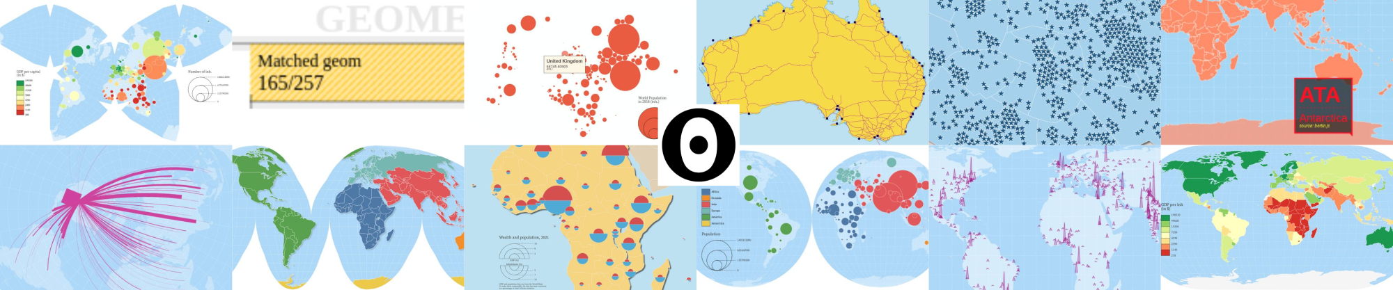
Bonus: an overview of available layer types
What's available in the bertin javascript library? What types of maps can be made? Thanks to this cheat sheet, you have an overview of the "types" available in the library. All these thumbnails are generated for real with the bertin@1.5.9 in this notebook.
