AWS Batch Simulator
Suppose you need to run heavy batch workloads, such as training ML models or running image processing algorithms on large files. These jobs are created as a result of your customers' actions, who operate independently of each other. This all makes it impossible to know exactly when a job will arrive to be processed. You also don't know exactly how long each job will take, as it depends on exactly what kind of computation each one carries out. But historical data tells you, on average, how many jobs arrive per hour and how long each job takes to run.
You are planning to implement this system on AWS Batch, describing the
necessary infrastructure with the CDK. In order to serve your traffic
properly, how many compute environments do you need? How much compute capacity
should they have? Is it better to use Fargate, ECS or EKS compute environments?
If using ECS or EKS, which allocation strategy is better: BEST_FIT or
BEST_FIT_PROGRESSIVE? What will happen if you need to add another job queue?
This library can help you answer all these questions by simulating traffic to your candidate infrastructure, from your computer, before you deploy anything to AWS.
Note All the logic implemented in this library is based on the behavior described in public AWS documents. However, there are many aspects of AWS Batch that are not public, and therefore cannot be modeled at all, such as the scaling time (how long it takes for a compute environment to go from min vCPUs to max vCPUs) or the transition times (how long it takes from a job to go from one state to the next). As a result, the values in the simulation report should not be taken as an accurate prediction of how the actual system will perform. Rather, you should consider those results relative to one another, to judge how different set-ups respond to the same traffic pattern.
Basic usage
Let's say you decide to start out with the following set-up: a single job queue, connected to a single Fargate compute environment, which can scale up to 60 vCPUs:
export class BatchApplicationStack extends cdk.Stack {
  constructor(scope: Construct, id: string, props?: cdk.StackProps) {
    super(scope, id, props);

    const vpc = new ec2.Vpc(this, 'myVpc');
    const environment = new batch.FargateComputeEnvironment(this, 'env', {
      vpc,
      maxvCpus: 60,
    });
    const queue: batch.JobQueue = new batch.JobQueue(this, 'myJobQueue');
    queue.addComputeEnvironment(environment, 1);
  }
}
And you want your jobs to run in containers with 4 dedicated vCPUs:
const jobDefinition = new batch.EcsJobDefinition(stack, 'ML-training', {
  container: new batch.EcsFargateContainerDefinition(stack, 'containerDef', {
    image: ecs.ContainerImage.fromRegistry('some-docker-image'),
    memory: Size.mebibytes(1024),
    cpu: 4,
  }),
});
In your CDK application entrypoint, you can simulate how this infrastructure
will handle traffic by creating a BatchSimulator, and using it to run a
simulation with the parameters you obtained empirically:
const app = new cdk.App();
const stack = new BatchApplicationStack(app, 'BatchApplication');

// Assuming a Markov process
const simulator = BatchSimulator.markov(stack);

// const jobDefinition = ... (as defined above)

app.synth();

const report = simulator.simulate([{
  jobDefinition,
  meanServiceTime: 15, // minutes
  arrivalRate: 0.9, // jobs/min = 54 jobs/h
}]);
In this example, the jobs arrive independently of each other at the queue at a rate of 54 jobs per hour (0.9 jobs/min), but they are not evenly distributed. Instead, the probability that $k$ jobs arrive in the next minute is given by a Poisson distribution:
$$ f(k; \lambda) = \Pr(X{=}k)= \frac{\lambda^k e^{-\lambda}}{k!} $$
where $\lambda = 0.9$, in our example, is the arrival rate. Likewise, the execution times (also known as "service times") are not uniformly distributed, but rather exponentially distributed:
$$ f(x;\lambda) = \lambda e^{ - \lambda x} $$
where $\lambda$ is the inverse of the mean service time. In this case, $\lambda = 1 / 15$.
This type of behavior is very common in queueing systems, and is known as a
"Markov process" (or "Markov chain"). Hence, BatchSimulator.markov(stack).
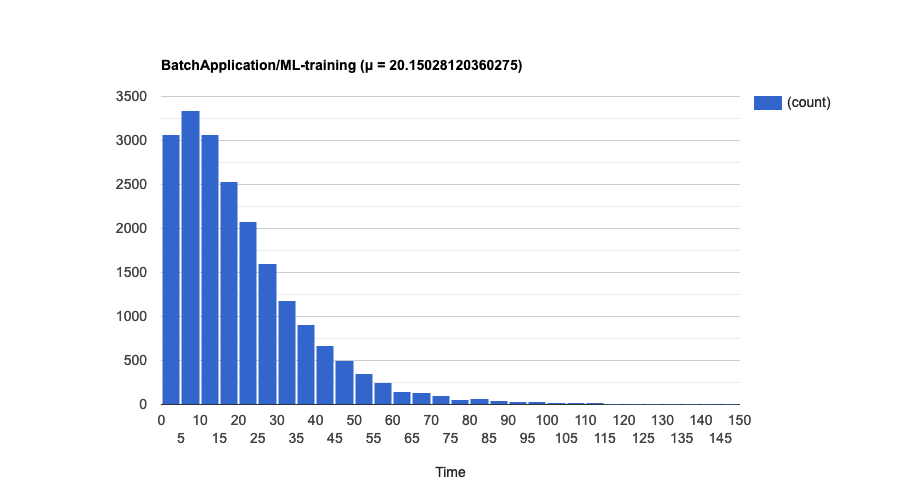
Notice that, in this example, we get a job almost every minute, but it takes 15 minutes for a job to execute (and thus leave the system, freeing up compute resources to execute the next job). If we were to process these jobs sequentially, the queue would grow indefinitely over time. Fortunately, the compute environment has 15 times the capacity needed to process such jobs ( an M/M/15 queue, in Kendall's notation). The simulation report tells us exactly how the service times are distributed:
The mean time in this particular simulation was about 20 minutes, compared to the average 15 minutes to run a job. The extra 5 minutes or so were spent by the jobs waiting in the queue.
The report also shows how congested the system was over the course of the simulation, indicated by the number of jobs in the queue at each point in time:
To get the HTML version of the simulation report, that includes these charts,
use the report.toHtml() method.
Fair-share scheduling
Now suppose that there are two departments in your company that can submit jobs of this type: Research and Finance, with Finance accounting for about 80% of the jobs submitted. You can model this scenario with weight factor probabilities:
const report = simulator.simulate([{
  jobDefinition: jobDefinition,
  meanServiceTime: 15,
  arrivalRate: 0.9,
  weightFactorProbabilities: {
    Research: 0.2,
    Finance: 0.8,
  },
}]);
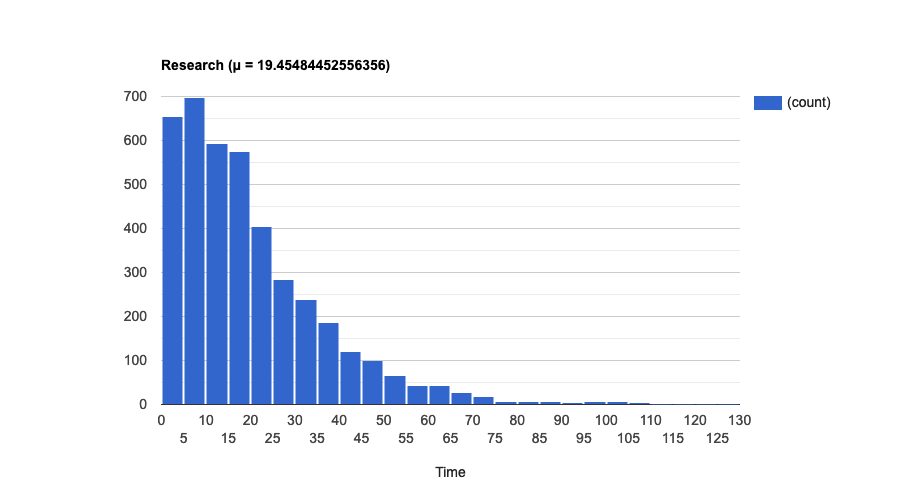
As the simulation report shows, both departments have to wait about the same amount of time (approximately 19.5 min), on average, for their jobs to finish. This is because the default scheduling policy for a job queue is first-in, first-out (FIFO), so every job, regardless of their share identifier, has to wait for the same number of jobs in the queue, on average.
But let's say you have a service level agreement with the Research department that the mean execution time from their perspective (from submission to completion) should be less than 18 min. One way to achieve this is by deprioritizing the Finance jobs, using fair-share scheduling instead of FIFO. By experimenting with different sets of values (and running a simulation for each one), we conclude that we can achieve the desired result by giving the Research jobs 8 times more weight than Finance jobs:
const queue: batch.JobQueue = new batch.JobQueue(this, 'myJobQueue', {
  schedulingPolicy: new batch.FairshareSchedulingPolicy(this, 'fairshare', {
    shares: [{
      shareIdentifier: 'Research',
      weightFactor: 1,
    }, {
      shareIdentifier: 'Finance',
      // weightFactor is inversely correlated with the number of vCPUs
      // allocated to a share identifier.
      weightFactor: 8,
    }],
  }),
});
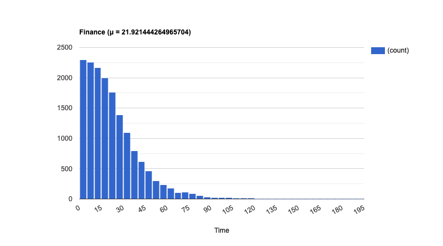
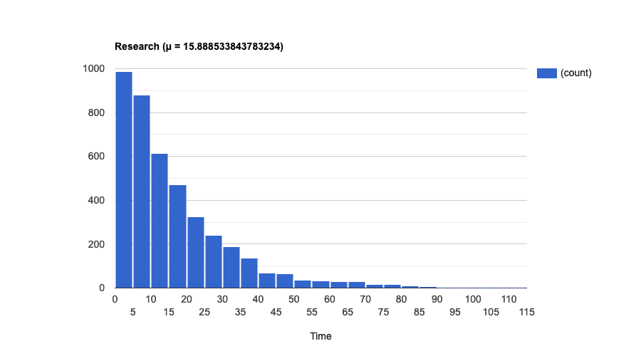
The resulting mean times are about 22 minutes for Finance and 16 minutes for Research:
Retry strategies
Let's go back to the basic example, and add a retry strategy, in which jobs that fail with a non-zero exit code are retried up to 2 times:
const jobDefinition = new batch.EcsJobDefinition(stack, 'ML-training', {
  container: new batch.EcsFargateContainerDefinition(stack, 'containerDef', {
    image: ecs.ContainerImage.fromRegistry('some-docker-image'),
    memory: Size.mebibytes(1024),
    cpu: 4,
  }),
  retryAttempts: 2,
  retryStrategies: [{
    action: Action.RETRY,
    on: Reason.NON_ZERO_EXIT_CODE
  }],
});
What happens if jobs of this definition have a 95% probability of success? Let's model this first:
const report = simulator.simulate([{
  jobDefinition: jobDefinition,
  meanServiceTime: 15,
  arrivalRate: 0.9,
  successProbability: 0.95,
}]);
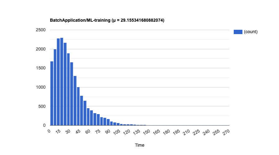
And then run a simulation, which shows that the mean time jumps to about 29 minutes, in this case:
At the moment, the simulator doesn't take into account the error reasons. In the
simulation, generated jobs that are considered to fail will be "retried"
if their job definition has at least one retry strategy with action RETRY.
Using other distributions
Although the Markov process is the most commonly used to model queueing systems,
your particular use case may be better modeled by some other process. For
example, in many applications, batch jobs are triggered periodically by some
scheduler like cron. The service time may still be exponentially distributed,
but the inter-arrival time is now deterministic. To model these situations, use
the lower-level API provided by the general process:
const simulator = BatchSimulator.general(stack);and specify the probability distributions directly:
const report = simulator.simulate([{
  jobDefinition: smallJob,
  interArrivalTimeDistribution: Distribution.deterministic(5),
  serviceTimeDistribution: Distribution.exponential(1 / 30),
}]);
In addition to deterministic and exponential distributions, the simulator also
offers an implementation of the Erlang distribution. But If you need to use
some probability distribution that is not available in the Distribution class,
you can bring your own, by implementing the IDistribution interface.
Unsupported features (yet)
Some of the AWS Batch features are not being simulated by this library:
- Queue priority: If you have multiple queues sharing a compute environment, they will be treated with the same priority. The order in which jobs will be picked for execution depends only on their position in, and the scheduling policies of, their respective queues.
-
Spot instances: The
spot: trueconfiguration in compute environments is completely ignored. - Share decay: Even though compute reservation is taken into account for simulation, the share decay, if defined, is also ignored.

