nurbs

Non-Uniform Rational B-Splines (NURBS) of any dimensionality

This library implements n-dimensional Non-Uniform Rational B-Splines (NURBS). It has no dependencies and uses code generation to unroll loops, optimize for various cases (uniform and non-uniform; rational and non-rational; clamped, open, and periodic) and allow compatibility with multiple input types (arrays of arrays, ndarrays). It's mainly concerned with evaluation as opposed to operations on the splines.

Installation

$ npm install nurbs

Overview

• Examples
  • Open B-Spline
  • Clamped B-Spline
  • Closed B-spline
  • Closed NURBS
  • Basis Functions
  • Derivatives
  • Transforms
  • Curves, Surfaces, Volumes, etc.
  • ndarrays
• API
  • nurbs
  • Properties
    • domain
    • splineDimension
    • dimension
    • size
  • Methods
    • evaluate
    • evaluator
    • support
    • transform

Examples

Open B-Spline

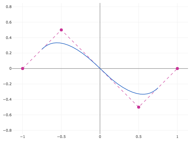
To construct an open quadratic B-Spline in two dimensions:

var nurbs = require('nurbs');
 
var curve = nurbs({
  points: [[-1, 0], [-0.5, 0.5], [0.5, -0.5], [1, 0]],
  degree: 2
});
 
curve.domain;
// => [[2, 4]]
 
curve.size;
// => [4]
 
curve.splineDimension;
// => 1
 
curve.dimension;
// => 2
 
curve.evaluate([], 3.0);
// => [0, 0]

If you don't provide a knot vector, a uniform knot vector with integer values will be provided implicitly. In this case the knots would be [0, 1, 2, 3, 4, 5, 6]. The above example queries the valid domain using curve.domain, which returns a nested array since each dimension is parameterized separately. In this case that's just one dimension, from t = 2 to t = 4. Plotting shows the open (unclamped) spline:

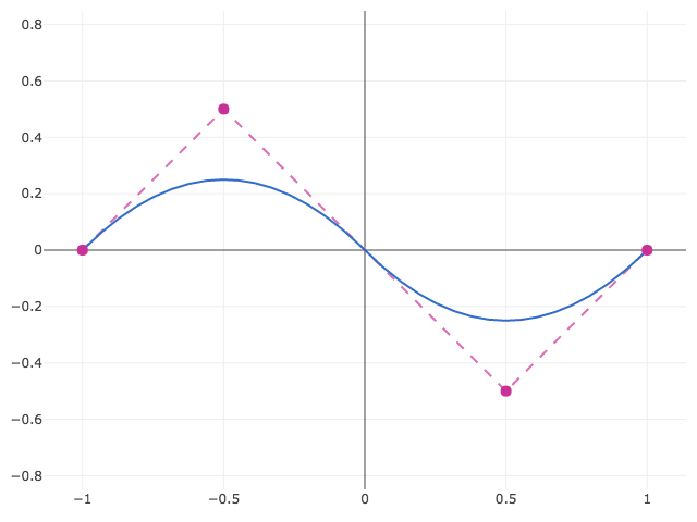
Clamped B-Spline

To construct a clamped spline, that is, a spline which passes through its endpoints, you may specify boundary conditions with the boundary property:

var curve = nurbs({
  points: [[-1, 0], [-0.5, 0.5], [0.5, -0.5], [1, 0]],
  degree: 2,
  boundary: 'clamped'
});
 
curve.domain;
// => [[2, 4]]

In this case the knots would be [2, 2, 2, 3, 4, 4, 4], where the particular range is a result of clamping of the open knot vector by repeating the first and last knots degree + 1 times. As a result, the domain [2, 4] is unchanged from the previous example.

To change the data of an existing spline instance, you could also call curve as a constructor, which will then reset and sanitize all of the data, as in curve({points: ..., degree: ..., ...}).

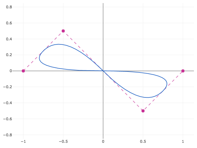
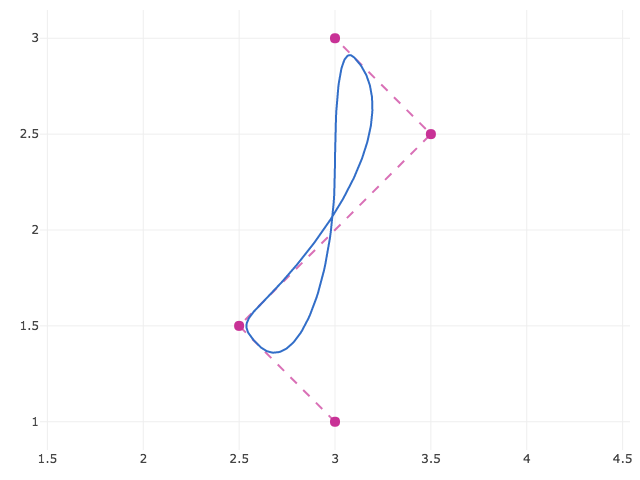
Closed B-Spline

A B-Spline can be made periodic by wrapping around and duplicating the first or last points a number of times equal to the degree. This library includes a 'closed' boundary condition so that a spline can be closed without explicit repitition. If knots are not provided, that start of a closed spline's domain becomes t = 0. The result contains the open spline from the first example with the same parameterization ([2, 4]) as well as a segment that closes the spline ([0, 2]).

var curve = nurbs({
  points: [[-1, 0], [-0.5, 0.5], [0.5, -0.5], [1, 0]],
  degree: 2,
  boundary: 'closed'
});
 
curve.domain;
// => [[0, 4]]

Plotting shows the closed spline:

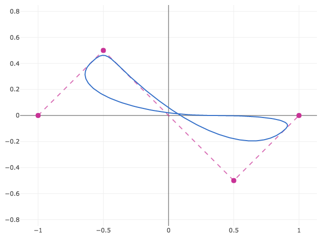
Closed NURBS

Going from B-Splines to NURBS means the addition of weights and non-uniform knots. Weights are straightforward since they correspond directly to points. As for knots, an unclosed NURBS spline requires n + degree + 1 knots, where n is the number of points. A closed NURBS curve requires only n + 1 knots. The periodicity is defined by equivalence of the first and last knot, i.e. k_0 := k_n. The knots then define n unique, periodic knot intervals. For example,

var curve = nurbs({
  points: [[-1, 0], [-0.5, 0.5], [0.5, -0.5], [1, 0]],
  weights: [0.5, 4, 1, 0.5],
  knots: [[0, 1, 3, 7, 15]],
  boundary: 'closed',
  degree: 2
});
 
curve.domain;
// => [[0, 15]]

Basis functions

A b-spline does not pass through its control points. If you want to do more advanced analysis such as constructing a spline that passes through a set of points, you may evaluate the basis functions directly. If you don't yet have a set of points defining the spline, you may initialize a spline with a size instead of a points. Then to determine the contribution at (u, v) = [1.3, 2.4] of the very first point, indexed by points[0][0]:

var curve = nurbs({size: [10, 15]});
var basis = curve.evaluator(null, true);
basis(1.3, 2.4, 0, 0);

You may also query which points contribute to a given parameter value with support:

curve.support([], 1.3, 2.4)

Derivatives

To evaluate a derivative, you may create an evaluator using the same method as for basis functions above. Derivatives are specified by order and per-dimension, so that the third derivative in the second dimension would be specified as:

var curve = nurbs({points: [[[...], ...], ...]});
var derivative = curve.evaluator([0, 3]);
derivative([], 1.3, 2.4);

Note that currently only first derivatives are implemented for non-uniform rational b-splines. Non-uniform (non-rational) b-splines support higher orders.

For simple curves, a non-array-wrapped derivative order is permitted so that the first derivative of a curve is simply:

var curve = nurbs({points: [...]});
var derivative = curve.evaluator(1);
derivative([], 1.3);

Transforms

Each nurbs object has a transform method that accepts a matrix using gl-matrix style matrices. See gl-mat2, gl-mat3, and gl-mat4. For example, to apply a transformation in-place to the previous example:

var mat3 = require('gl-mat3');
var m = mat3.identity([]);
mat3.translate(m, m, [3, 2, 0]);
mat3.rotate(m, m, Math.PI / 2);
curve.transform(m);

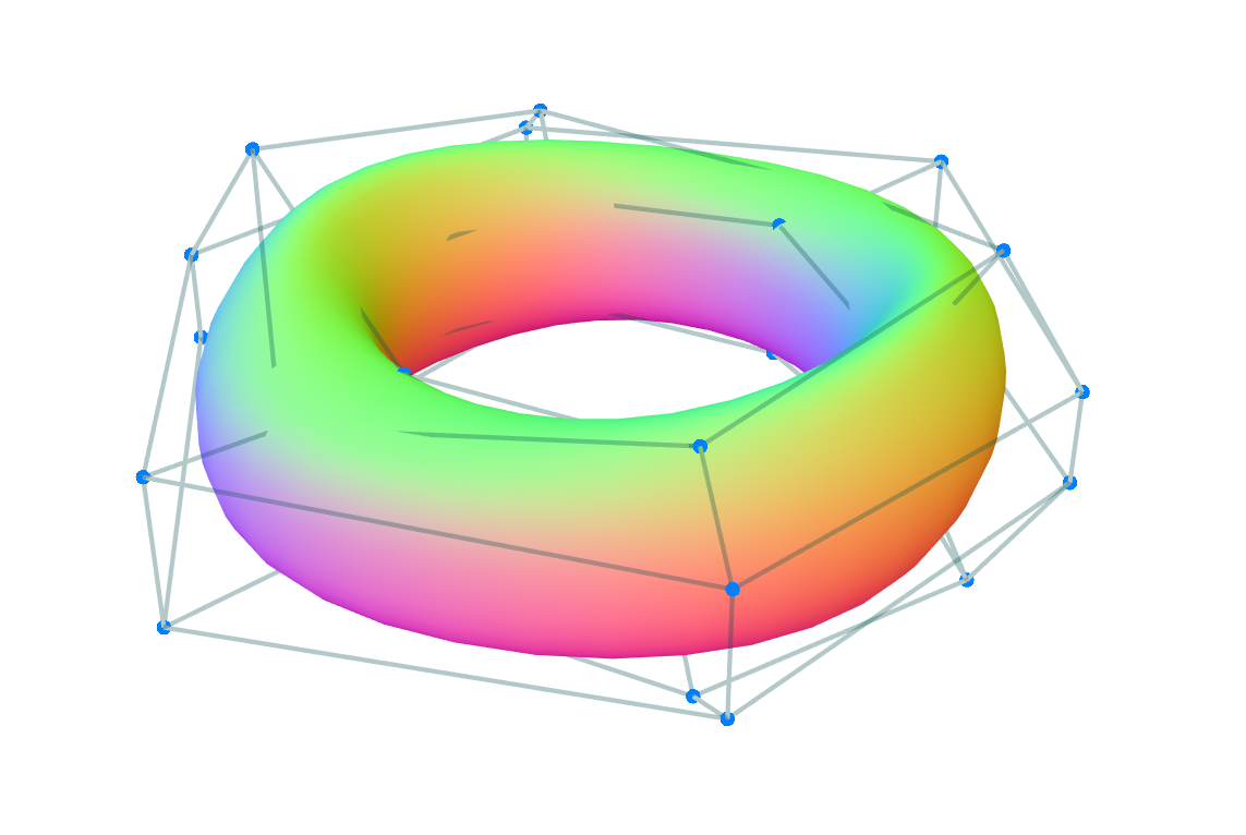
Curves, Surfaces, Volumes, etc.

The above concepts generalize to any dimensionality of spline surface and space dimensions. You can create a surface patch in three dimensions using the code below. In this case, each property is specified per-dimension.

var curve = nurbs({
  points: [
    [[0, 2, 3], [4, 5, 6], [7, 8, 9]],
    [[1, 2, 2], [1, 2, 3], [4, 5, 6]],
    [[1, 2, 2], [1, 2, 3], [4, 5, 6]],
    [[1, 2, 2], [1, 2, 3], [4, 5, 6]],
  ],
  weights: [
    [2, 1, 1],
    [2, 2, 1],
    [2, 3, 1],
    [2, 2, 1]
  ],
  knots: [
    [0, 0, 0, 0, 0.5, 1, 1, 1, 1],
    [0, 0, 0, 1, 1, 1]
  ],
  boundary: ['closed', 'clamped'],
  degree: [3, 2],
});
 
curve.evaluate([], 0.5, 0.5);

examples/3d.js shows a 3D surface created in this way using the regl library. See the live version here.

ndarrays

Arrays of arrays are easy to work with for dynamically inserting and removing points, but may be problematic due to access and the allocation of many small arrays. points and weights also accept ndarrays (either array or typed array backed or generic get/set ndarrays). The object does not need to be an actual ndarray. Any object is acceptable as long as it has ndarray-style data, shape, stride, and offset properties. This also means that if you have packed vertex data, you can trivially wrap it in an ndarray-style object.

The ndarray-pack module is a simple way to see the correspondence between array of arrays and ndarrays:

var pack = require('ndarray-pack');
 
var points = [
  [[0, 2, 3], [4, 5, 6], [7, 8, 9]],
  [[1, 2, 2], [1, 2, 3], [4, 5, 6]],
  [[1, 2, 2], [1, 2, 3], [4, 5, 6]],
];
 
// These two are equivalent:
var curve1 = nurbs(pack(points));
var curve2 = nurbs(points);

API

nurbs(points, degree, weights, knots, boundary, options)

nurbs(options)

Construct a NURBS object. Options are:

• points (optional): An array of arrays or ndarray-style object containing control points.

  If an array of arrays, the length of points corresponds to the number of points in the first spline dimension, the lenth of points[0] to the number of points in the second spline dimension, and so on. The number of components in the innermost array corresponds to the spatial dimension of the spline. For example, [[[1, 2, 3], [4, 5, 6]], [[7, 8, 9], [10, 11, 12]]] corresponds to a surface in three dimensions.

  If an ndarray, three variants are permitted.

  • Regular ndarrays backed by an array or typed array of data.
  • Generic ndarrays backed by get and set methods.
  • ndarray-like object containing data, shape, stride, and offset properties.

  Note that providing data as an ndarray is equivalent to running ndarray-pack on array-of-arrays-style data.

  If points is ommitted, then a size must be provided instead.

• weights (optional): An array of arrays or ndarray-style object containing control point weights. If not provided, the weight computation is omitted, which is equivalent to all weights equal to 1.

• degree (optional, default 2): Either an integer degree or an array of integer degrees for each spline dimension. Must be less than the number of points. If a degree is specified and insufficient points are provided, an error will be thrown. If the degree is unspecified and insufficient points are provided (i.e. two points), the degree will be downgraded to 1.

• knots (optional): An array of knot vector arrays for each respective spline dimension. Each knot vector is presumed to be strictly nondecreasing.

• boundary (optional, default 'open'): An array of boundary conditions for each spline dimension or single non-array-wrapped boundary condition to be applied to all dimensions. Options are:

  • 'clamped': a spline that meets the control points at each end.
  • 'open': an evenly spaced knot vector such that the spline does not meet the control points
  • 'closed': equal to an open spline wherever the open spline is defined, with an additional section closing the gap to create a closed loop.

  Note that clamped on one end and open on the other is perfectly possible but requires specifying your own knot vector.

• options (optional): An object containing additional configuration options. Permitted options are:

  • debug (boolean, default false): When true, writes the generated code to the console.
  • checkBounds (boolean, default false): When true, checks each parameter against the dimension's domain and throws an error if a point outside the defined domain is evaluated. Behavior is undefined otherwise.
  • size (array): if you only wish to evaluate the basis functions, you may omit points and provide an array containing the number of points in the control hull in each respective spline dimension. For example, a 5 × 3 control hull would be size: [5, 3].

Properties

spline.domain

An array of arrays containing the minimum and maximum spline parameters for each respective spline dimension.

---

spline.splineDimension

Dimensionality of the spline surface, e.g. curve = 1, surface = 2, etc.

---

spline.dimension

Spatial dimension of the spline. One-dimensional = 1, 2D plane = 2, etc.

---

spline.size

Size of the control point data.

Methods

spline.evaluate(out, t0, t1, ..., tn_1)

Evaluate the spline at the parameters t₀, ..., t_{n - 1} where n is the dimensionality of the surface (i.e. curve = 1, surface = 2, etc), and write the result to out. Returns a reference to out.

---

spline.evaluator(derivativeOrders, isBasis)

Returns a function which evaluates the spline according to the specified arguments. spline.evaluate is just the special case spline.evaluator(null, false).

Arguments are:

• derivativeOrders (Number or Array of Numbers, default: undefined): If provided, evaluates the corresponding partial derivative. For example, to evaluate the third derivative in the second dimension of a spline, you would call spline.evaluator([0, 3]). See [1] for more details.

  Currently only first derivatives are implemented for non-uniform rational b-splines. Non-uniform (non-rational) b-splines support higher orders.

• isBasis (boolean, default: false): If true, creates a basis function evaluator instead of a direct spline evaluator. Returns a function function basis(t0, t1, ..., tn_1, i0, i1, ..., in_1) (no out argument is necessary since the answer is always a scalar) which evaluates the value of the spline basis functions for a given parameter location and control hull indices. The inputs t0, ..., tn_1 are the spline parameters (t₀, t₁, ..., t_{n - 1}) and the indices i0, ..., in_1 are the integer indices of a control point (i₀, i₁, ..., i_{n - 1}). The output is a real number between 0 and 1 by which the correpsonding control point is multiplied. Summing across all points in the spline.support gives the computed spline position. When possible, evaluating the spline directly is much faster.

---

spline.support(out, t0, t1, ..., tn_1)

Compute the support of a point on the spline. That is, the integer indices of all control points that influence the spline at the given position. To avoid allocation of many small arrays, the result is written in-place to array out as a packed array of index tuples, e.g. indices [0, 5, 3] and [1, 5, 3] are returned as [0, 5, 3, 1, 5, 3]. Returns a reference to out.

---

spline.transform(m)

Transform a spline in-place using gl-matrix-style matrices (e.g. gl-mat3 or gl-mat4). Modifies spline data and returns a reference to the spline.

References

• [1] Floater, M. S. Evaluation and Properties of the Derivative of a NURBS Curve. Mathematical Methods in Computer Aided Geometric Design II 261–274 (1992). doi:10.1016/b978-0-12-460510-7.50023-9

Credits

Development supported by Standard Cyborg.

License

© 2018 Standard Cyborg, Inc. MIT License.